机器学习作业第一周
这是吴恩达老师的机器学习作业....并不是我们学校的 hh
因为机器学习这个课是老师在2014年讲的,那时候Python还不火,所以老师讲的时候用的是ocatve,现在我准备都用Python写.
总结
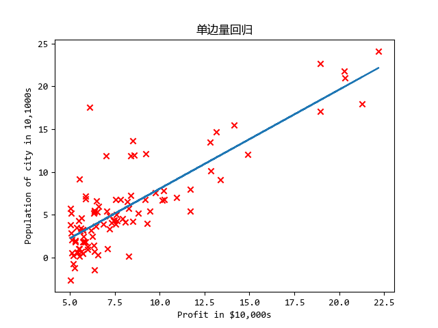
这是第一周作业,单/多变量线性回归
注意损失函数求导出来的结果,更新方式是不一样的
python中的矩阵和list类型非常蛋疼,不如matlab全是矩阵就好了给X加列,可以利用矩阵乘法快速求解
绘3维图时要用
meshgrid函数连接变量numpy.std函数要加上参数ddof=1,因为他的标准差默认除以n
重要公式的推导
这里有一个多变量的梯度更新,需要把原来的损失函数进行求导,因为现在是每一个变量都是向量,所以推导的时候我纠结了好一会。具体如下:
注:上标为行数,下标为列数,设数据X=[m,n]
\[ \begin{aligned} \theta_j &= \theta_j - \alpha\frac{\partial}{\partial\theta_j}J(\theta) = \theta_j - \alpha\frac{1}{m}\sum_{i=1}^{m}(h_\theta(x^{(i)}) - y^{(i)})*x_j^{(i)} \\ \theta_j &-=\frac{ \alpha}{m}\sum_{i=1}^{m}(h_\theta(x^{(i)}) - y^{(i)})*x_j^{(i)} \end{aligned} \] 现在我们分析此部分\(\sum_{i=1}^{m}(h_\theta(x^{(i)}) - y^{(i)})*x_j^{(i)}\):
注:以下都省略了常数项\(\alpha/m\)
\[ \begin{aligned} \because &x=[m,n]\ \ \ y=[m,1]\\ \therefore &x^{(i)} =[1,n]\ \ \ y^{(i)}=[1,1]\ \ \ \theta=[n,1] \\ \Rightarrow &h_\theta(x^{(i)})=x^{(i)}*\theta=[1,1]\\ \Rightarrow &h_\theta(x^{(i)})-y^{(i)}=[1,1]=E_\theta^{(i)}\\ \because &\sum_{i=1}^{m}(h_\theta(x^{(i)}) - y^{(i)})*x_j^{(i)}=\sum_{i=1}^{m}E_\theta^{(i)}*x_j^{(i)}\\ &=E_\theta^{(0)}*x_j^{(0)}+E_\theta^{(1)}*x_j^{(1)}+\ldots+E_\theta^{(m)}*x_j^{(m)}\\ \therefore \Theta&= \begin{bmatrix} x_1^1E_1 + x_2^1E_1 + \ldots + x_m^1E_1 \\ x_1^2E_2 + x_2^2E_2 + \ldots + x_m^2E_2 \\ x_1^nE_n + x_2^nE_n + \ldots + x_m^nE_n \\ \end{bmatrix} \end{aligned} \]
将其放到全局的矩阵中就是这样:
\[ \begin{aligned} X&=\begin{bmatrix} x_1^1 & x_2^1 & \ldots & x_n^1 \\ \vdots & \vdots & \ldots & \vdots \\ x_1^m & x_2^m & \ldots & x_n^1 \\ \end{bmatrix}\\ Y&=\begin{bmatrix} y_1^1 \\ \vdots \\ y_1^m \\ \end{bmatrix}\\ \theta&=\begin{bmatrix} \theta_1^1 \\ \vdots \\ \theta_1^n \\ \end{bmatrix} \\ \Theta-&=X^T(h_\theta(X) -Y) = X^T(X*\Theta-Y) \\ &= \begin{bmatrix} x_1^1 & x_1^2 & \ldots & x_1^m \\ \vdots & \vdots & \ldots & \vdots \\ x_n^1 & x_n^2 & \ldots & x_n^m \\ \end{bmatrix}* (\begin{bmatrix} x_1^1 & x_2^1 & \ldots & x_n^1 \\ \vdots & \vdots & \ldots & \vdots \\ x_1^m & x_2^m & \ldots & x_n^1 \\ \end{bmatrix}* \begin{bmatrix} \theta_1^1 \\ \vdots \\ \theta_1^n \\ \end{bmatrix}- \begin{bmatrix} y_1^1 \\ \vdots \\ y_1^m \\ \end{bmatrix}) \\ &= \begin{bmatrix} x_1^1 & x_1^2 & \ldots & x_1^m \\ \vdots & \vdots & \ldots & \vdots \\ x_n^1 & x_n^2 & \ldots & x_n^m \\ \end{bmatrix}* \begin{bmatrix} h_1^1 - y_1^1 \\ \vdots \\ h_1^m - y_1^m \\ \end{bmatrix}\\ &= \begin{bmatrix} x_1^1E_1 + x_2^1E_1 + \ldots + x_m^1E_1 \\ x_1^2E_2 + x_2^2E_2 + \ldots + x_m^2E_2 \\ x_1^nE_n + x_2^nE_n + \ldots + x_m^nE_n \\ \end{bmatrix} \end{aligned} \]
即推出:
\[\Theta-=\frac{\alpha}{m}X^T(X*\Theta-Y)\] # 代码
import matplotlib.pyplot as plt |
执行:
➜ Machine_learning /usr/bin/python3 /media/zqh/程序与工程/Python_study/Machine_learning/machine_learning_exam/week1/ex1.py |
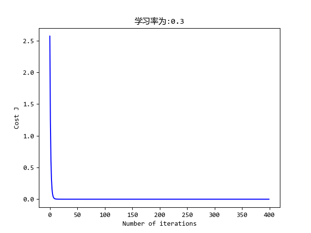
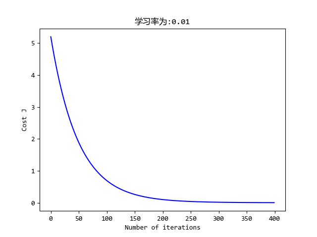
效果