机器学习作业第七周

这周是无监督学习算法,比较简单.k means之前就已经写过了,PCA主要是有个矩阵的奇异值分解需要看看矩阵相关知识.

ex7.py

from numpy.core import *
from scipy.io import loadmat
from imageio import imread
from sklearn import svm
import matplotlib.pyplot as plt
from fucs7 import findClosestCentroids, computeCentroids, runkMeans,\
    kMeansInitCentroids
if __name__ == "__main__":
    # Machine Learning Online Class
    #  Exercise 7 | Principle Component Analysis and K-Means Clustering
    #
    #  Instructions
    #  ------------
    #
    #  This file contains code that helps you get started on the
    #  exercise. You will need to complete the following functions:
    #
    #     pca.m
    #     projectData.m
    #     recoverData.m
    #     computeCentroids.m
    #     findClosestCentroids.m
    #     kMeansInitCentroids.m
    #
    #  For this exercise, you will not need to change any code in this file,
    #  or any other files other than those mentioned above.
    #

    # Initialization

    # ================= Part 1: Find Closest Centroids ====================
    #  To help you implement K-Means, we have divided the learning algorithm
    #  into two functions -- findClosestCentroids and computeCentroids. In this
    #  part, you shoudl complete the code in the findClosestCentroids function.
    #
    print('Finding closest centroids.')

    # Load an example dataset that we will be using
    data = loadmat('ex7data2.mat')
    X = data['X']  # [300,2]

    # Select an initial set of centroids
    K = 3  # 3 Centroids
    initial_centroids = array([
        [3., 3.],
        [6., 2.],
        [8., 5.]])

    # Find the closest centroids for the examples using the
    # initial_centroids
    idx = findClosestCentroids(X, initial_centroids)

    print('Closest centroids for the first 3 examples: ')
    print(idx[0: 3])
    print('\n(the closest centroids should be 0, 2, 1 respectively)')

    print('Program paused. Press enter to continue.')

    # ===================== Part 2: Compute Means =========================
    #  After implementing the closest centroids function, you should now
    #  complete the computeCentroids function.
    #
    print('\nComputing centroids means.')

    #  Compute means based on the closest centroids found in the previous part.
    centroids = computeCentroids(X, idx, K)

    print('Centroids computed after initial finding of closest centroids: ')
    print(centroids)
    print('\n(the centroids should be')
    print('   [ 2.428301 3.157924 ]')
    print('   [ 5.813503 2.633656 ]')
    print('   [ 7.119387 3.616684 ]')

    print('Program paused. Press enter to continue.')

    # =================== Part 3: K-Means Clustering ======================
    #  After you have completed the two functions computeCentroids and
    #  findClosestCentroids, you have all the necessary pieces to run the
    #  kMeans algorithm. In this part, you will run the K-Means algorithm on
    #  the example dataset we have provided.
    #
    print('\nRunning K-Means clustering on example dataset.')

    # Load an example dataset
    data = loadmat('ex7data2.mat')
    X = data['X']
    # Settings for running K-Means
    K = 3
    max_iters = 10

    # For consistency, here we set centroids to specific values
    # but in practice you want to generate them automatically, such as by
    # settings them to be random examples (as can be seen in
    # kMeansInitCentroids).
    initial_centroids = array(
        [[3., 3.],
         [6., 2.],
         [8., 5.]])

    # Run K-Means algorithm. The 'true' at the end tells our function to plot
    # the progress of K-Means
    centroids, idx = runkMeans(X, initial_centroids, max_iters, True)
    print('\nK-Means Done.')

    print('Program paused. Press enter to continue.')

    # ============= Part 4: K-Means Clustering on Pixels ===============
    #  In this exercise, you will use K-Means to compress an image. To do this,
    #  you will first run K-Means on the colors of the pixels in the image and
    #  then you will map each pixel on to it's closest centroid.
    #
    #  You should now complete the code in kMeansInitCentroids.m
    #

    print('\nRunning K-Means clustering on pixels from an image.')

    #  Load an image of a bird
    A = double(imread('bird_small.png'))

    # If imread does not work for you, you can try instead
    #   load ('bird_small.mat');

    A = A / 255  # Divide by 255 so that all values are in the range 0 - 1

    # Size of the image
    img_size = shape(A)

    # Reshape the image into an Nx3 matrix where N = number of pixels.
    # Each row will contain the Red, Green and Blue pixel values
    # This gives us our dataset matrix X that we will use K-Means on.
    X = reshape(A, (img_size[0] * img_size[1], 3))

    # Run your K-Means algorithm on this data
    # You should try different values of K and max_iters here
    K = 16
    max_iters = 10

    # When using K-Means, it is important the initialize the centroids
    # randomly.
    # You should complete the code in kMeansInitCentroids.m before proceeding
    initial_centroids = kMeansInitCentroids(X, K)

    # Run K-Means
    [centroids, idx] = runkMeans(X, initial_centroids, max_iters)

    print('Program paused. Press enter to continue.')

    # ================= Part 5: Image Compression ======================
    #  In this part of the exercise, you will use the clusters of K-Means to
    #  compress an image. To do this, we first find the closest clusters for
    #  each example. After that, we

    print('\nApplying K-Means to compress an image.')

    # Find closest cluster members
    idx = findClosestCentroids(X, centroids)

    # Essentially, now we have represented the image X as in terms of the
    # indices in idx.

    # We can now recover the image from the indices (idx) by mapping each pixel
    # (specified by it's index in idx) to the centroid value
    X_recovered = centroids[idx, :]

    # Reshape the recovered image into proper dimensions
    X_recovered = reshape(X_recovered, (img_size[0], img_size[0], 3))

    # Display the original image
    plt.figure()
    plt.subplot(1, 2, 1)
    plt.imshow(A)
    plt.title('Original')

    # Display compressed image side by side
    plt.subplot(1, 2, 2)
    plt.imshow(X_recovered)
    plt.title('Compressed, with {} colors.'.format(K))

    print('Program paused. Press enter to continue.')
    plt.show()

效果

Finding closest centroids.
Closest centroids for the first 3 examples:
[0 2 1]

(the closest centroids should be 0, 2, 1 respectively)
Program paused. Press enter to continue.

Computing centroids means.
Centroids computed after initial finding of closest centroids:
[[2.42830111 3.15792418]
 [5.81350331 2.63365645]
 [7.11938687 3.6166844 ]]

(the centroids should be
   [ 2.428301 3.157924 ]
   [ 5.813503 2.633656 ]
   [ 7.119387 3.616684 ]
Program paused. Press enter to continue.

Running K-Means clustering on example dataset.
K-Means iteration 0/10...

K-Means iteration 1/10...

K-Means iteration 2/10...

K-Means iteration 3/10...

K-Means iteration 4/10...

K-Means iteration 5/10...

K-Means iteration 6/10...

K-Means iteration 7/10...

K-Means iteration 8/10...

K-Means iteration 9/10...


K-Means Done.
Program paused. Press enter to continue.

Running K-Means clustering on pixels from an image.
K-Means iteration 0/10...

K-Means iteration 1/10...

K-Means iteration 2/10...

K-Means iteration 3/10...

K-Means iteration 4/10...

K-Means iteration 5/10...

K-Means iteration 6/10...

K-Means iteration 7/10...

K-Means iteration 8/10...

K-Means iteration 9/10...

Program paused. Press enter to continue.

Applying K-Means to compress an image.
Program paused. Press enter to continue.

ex7_pca.py

from numpy.core import *
from numpy.random import rand, randint
from scipy.io import loadmat
from sklearn import svm
from imageio import imread
import matplotlib.pyplot as plt
from mpl_toolkits.mplot3d import Axes3D
from fucs7 import featureNormalize, pca, drawline, projectData, recoverData,\
    displayData, runkMeans, kMeansInitCentroids, plotDataPoints

if __name__ == "__main__":
    # Machine Learning Online Class
    #  Exercise 7 | Principle Component Analysis and K-Means Clustering
    #
    #  Instructions
    #  ------------
    #
    #  This file contains code that helps you get started on the
    #  exercise. You will need to complete the following functions:
    #
    #     pca.m
    #     projectData.m
    #     recoverData.m
    #     computeCentroids.m
    #     findClosestCentroids.m
    #     kMeansInitCentroids.m
    #
    #  For this exercise, you will not need to change any code in this file,
    #  or any other files other than those mentioned above.
    #

    # ================== Part 1: Load Example Dataset  ===================
    #  We start this exercise by using a small dataset that is easily to
    #  visualize
    #
    print('Visualizing example dataset for PCA.\n\n')

    #  The following command loads the dataset. You should now have the
    #  variable X in your environment
    data = loadmat('ex7data1.mat')
    X = data['X']
    #  Visualize the example dataset
    plt.figure()
    plt.plot(X[:, 0], X[:, 1], 'bo')
    plt.axis([0.5, 6.5, 2, 8])
    # axis square

    print('Program paused. Press enter to continue.\n')
    # pause

    # =============== Part 2: Principal Component Analysis ===============
    #  You should now implement PCA, a dimension reduction technique. You
    #  should complete the code in pca.m
    #
    print('\nRunning PCA on example dataset.\n\n')

    #  Before running PCA, it is important to first normalize X
    X_norm, mu, sigma = featureNormalize(X)

    #  Run PCA
    U, S = pca(X_norm)

    #  Compute mu, the mean of the each feature

    #  Draw the eigenvectors centered at mean of data. These lines show the
    #  directions of maximum variations in the dataset.
    drawline(mu, mu + 1.5 * S[0, 0]*U[:, 0], 'k-')
    drawline(mu, mu + 1.5 * S[1, 1]*U[:, 1], 'k-')

    print('Top eigenvector: \n')
    print(' U[:,0] = {} {} \n'.format(U[0, 0], U[1, 0]))
    print('\n(you should expect to see -0.707107 -0.707107)\n')

    print('Program paused. Press enter to continue.\n')

    # =================== Part 3: Dimension Reduction ===================
    #  You should now implement the projection step to map the data onto the
    #  first k eigenvectors. The code will then plot the data in this reduced
    #  dimensional space.  This will show you what the data looks like when
    #  using only the corresponding eigenvectors to reconstruct it.
    #
    #  You should complete the code in projectData.m
    #
    print('\nDimension reduction on example dataset.\n\n')

    #  Plot the normalized dataset (returned from pca)
    plt.figure()
    plt.plot(X_norm[:, 0], X_norm[:, 1], 'bo')
    plt.axis([-4, 3, - 4, 3])

    #  Project the data onto K = 1 dimension
    K = 1
    Z = projectData(X_norm, U, K)
    print('Projection of the first example: {}\n'.format(Z[1]))
    print('\n(this value should be about 1.481274)\n\n')

    X_rec = recoverData(Z, U, K)
    print('Approximation of the first example: {} {}\n'.format(
          X_rec[0, 0], X_rec[0, 1]))
    print('\n(this value should be about  -1.047419 -1.047419)\n\n')

    #  Draw lines connecting the projected points to the original points
    plt.plot(X_rec[:, 0], X_rec[:, 1], 'ro')
    for i in range(size(X_norm, 0)):
        drawline(X_norm[i, :], X_rec[i, :], 'k--')

    print('Program paused. Press enter to continue.\n')
    # pause

    # =============== Part 4: Loading and Visualizing Face Data =============
    #  We start the exercise by first loading and visualizing the dataset.
    #  The following code will load the dataset into your environment
    #
    print('\nLoading face dataset.\n\n')

    #  Load Face dataset
    data = loadmat('ex7faces.mat')
    X = data['X']
    #  Display the first 100 faces in the dataset
    plt.figure()
    displayData(X[:99, :])

    print('Program paused. Press enter to continue.\n')

    # =========== Part 5: PCA on Face Data: Eigenfaces  ===================
    #  Run PCA and visualize the eigenvectors which are in this case eigenfaces
    #  We display the first 36 eigenfaces.
    #
    print('\nRunning PCA on face dataset.\n\
(this mght take a minute or two ...)\n\n')

    #  Before running PCA, it is important to first normalize X by subtracting
    #  the mean value from each feature
    X_norm, mu, sigma = featureNormalize(X)

    #  Run PCA
    U, S = pca(X_norm)

    #  Visualize the top 36 eigenvectors found
    displayData(U[:, :36].T)

    print('Program paused. Press enter to continue.\n')
    # pause

    # ============= Part 6: Dimension Reduction for Faces =================
    #  Project images to the eigen space using the top k eigenvectors
    #  If you are applying a machine learning algorithm
    print('\nDimension reduction for face dataset.\n\n')

    K = 100
    Z = projectData(X_norm, U, K)

    print('The projected data Z has a size of: ')
    print(shape(Z))

    print('\n\nProgram paused. Press enter to continue.\n')
    # pause

    # ==== Part 7: Visualization of Faces after PCA Dimension Reduction ====
    #  Project images to the eigen space using the top K eigen vectors and
    #  visualize only using those K dimensions
    #  Compare to the original input, which is also displayed

    print('\nVisualizing the projected (reduced dimension) faces.\n\n')

    K = 100
    X_rec = recoverData(Z, U, K)

    # Display normalized data
    plt.figure()
    plt.subplot(1, 2, 1)
    displayData(X_norm[:100, :])
    plt.title('Original faces')

    # Display reconstructed data from only k eigenfaces
    plt.subplot(1, 2, 2)
    displayData(X_rec[:100, :])
    plt.title('Recovered faces')

    print('Program paused. Press enter to continue.\n')
    # pause

    # === Part 8(a): Optional (ungraded) Exercise: PCA for Visualization ===
    #  One useful application of PCA is to use it to visualize high-dimensional
    #  data. In the last K-Means exercise you ran K-Means on 3-dimensional
    #  pixel colors of an image. We first visualize this output in 3D, and then
    #  apply PCA to obtain a visualization in 2D.

    # Re-load the image from the previous exercise and run K-Means on it
    # For this to work, you need to complete the K-Means assignment first
    A = double(imread('bird_small.png'))

    # If imread does not work for you, you can try instead
    #   load ('bird_small.mat');

    A = A / 255
    img_size = shape(A)
    X = reshape(A, (img_size[0] * img_size[1], 3))
    K = 16
    max_iters = 10
    initial_centroids = kMeansInitCentroids(X, K)
    centroids, idx = runkMeans(X, initial_centroids, max_iters)

    #  Sample 1000 random indexes (since working with all the data is
    #  too expensive. If you have a fast computer, you may increase this.
    sel = randint(size(X, 0), size=1000, dtype=int)

    #  Setup Color Palette
    # palette = hsv(K)
    # colors = palette(idx(sel), :)

    #  Visualize the data and centroid memberships in 3D
    fig = plt.figure()
    ax = fig.add_subplot(111, projection='3d')
    ax.scatter(X[sel, 0], X[sel, 1], X[sel, 2],  c=idx[sel] % K)
    plt.title('Pixel dataset plotted in 3D. Color shows centroid memberships')

    print('Program paused. Press enter to continue.\n')

    # === Part 8(b): Optional (ungraded) Exercise: PCA for Visualization ===
    # Use PCA to project this cloud to 2D for visualization

    # Subtract the mean to use PCA
    X_norm, mu, sigma = featureNormalize(X)

    # PCA and project the data to 2D
    U, S = pca(X_norm)
    Z = projectData(X_norm, U, 2)

    # Plot in 2D
    plt.figure()
    plotDataPoints(Z[sel, :], idx[sel], K)
    plt.title('Pixel dataset plotted in 2D, using PCA for dimensionality reduction')
    print('Program paused. Press enter to continue.\n')
    plt.show()

效果

Visualizing example dataset for PCA.

Program paused. Press enter to continue.
Running PCA on example dataset.

Top eigenvector:
 U[:,0] = -0.7071067811865472 -0.7071067811865475
(you should expect to see -0.707107 -0.707107)
Program paused. Press enter to continue.
Dimension reduction on example dataset.

Projection of the first example: [1.48127391]
(this value should be about 1.481274)

Approximation of the first example: -1.0474188259204957 -1.047418825920496
(this value should be about  -1.047419 -1.047419)

Program paused. Press enter to continue.
Loading face dataset.

Program paused. Press enter to continue.
Running PCA on face dataset.
(this mght take a minute or two ...)

Program paused. Press enter to continue.
Dimension reduction for face dataset.

The projected data Z has a size of:
(5000, 100)

Program paused. Press enter to continue.
Visualizing the projected (reduced dimension) faces.

Program paused. Press enter to continue.
K-Means iteration 0/10...

K-Means iteration 1/10...

K-Means iteration 2/10...

K-Means iteration 3/10...

K-Means iteration 4/10...

K-Means iteration 5/10...

K-Means iteration 6/10...

K-Means iteration 7/10...

K-Means iteration 8/10...

K-Means iteration 9/10...

Program paused. Press enter to continue.
Program paused. Press enter to continue.

fucsy.py

from numpy.core import *
from numpy import r_, c_, diag
from numpy.random import permutation
from numpy.linalg import svd
from numpy.matrixlib import mat
import matplotlib.pyplot as plt
from scipy.spatial.distance import cdist


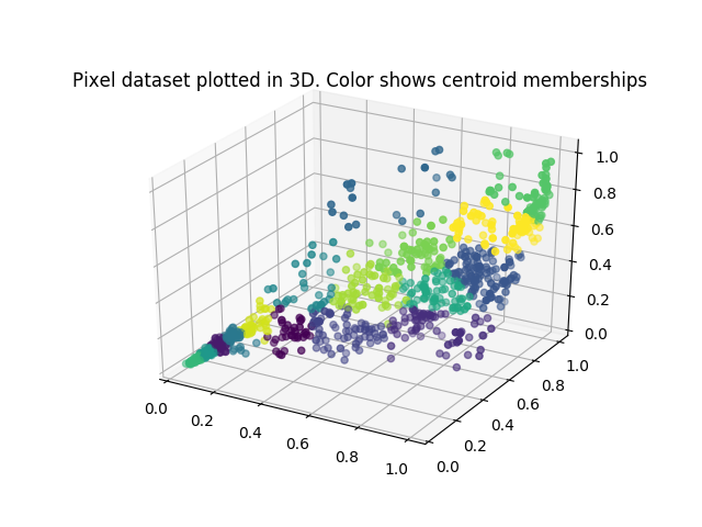
def findClosestCentroids(X: ndarray, centroids: ndarray):
    # FINDCLOSESTCENTROIDS computes the centroid memberships for every example
    #   idx = FINDCLOSESTCENTROIDS (X, centroids) returns the closest centroids
    #   in idx for a dataset X where each row is a single example. idx = m x 1
    #   vector of centroid assignments (i.e. each entry in range [1..K])
    #

    # Set K
    K = size(centroids, 0)

    # You need to return the following variables correctly.
    idx = zeros((size(X, 0), 1))

    # ====================== YOUR CODE HERE ======================
    # Instructions: Go over every example, find its closest centroid, and store
    #               the index inside idx at the appropriate location.
    #               Concretely, idx(i) should contain the index of the centroid
    #               closest to example i. Hence, it should be a value in the
    #               range 1..K
    #
    # Note: You can use a for-loop over the examples to compute this.
    #

    idx = argmin(cdist(X, centroids), axis=1)

    # =============================================================

    return idx  # 1d array


def computeCentroids(X: ndarray, idx: ndarray, K: int):
    # COMPUTECENTROIDS returs the new centroids by computing the means of the
    # data points assigned to each centroid.
    #   centroids = COMPUTECENTROIDS(X, idx, K) returns the new centroids by
    #   computing the means of the data points assigned to each centroid. It is
    #   given a dataset X where each row is a single data point, a vector
    #   idx of centroid assignments (i.e. each entry in range [1..K]) for each
    #   example, and K, the number of centroids. You should return a matrix
    #   centroids, where each row of centroids is the mean of the data points
    #   assigned to it.
    #

    # Useful variables
    m, n = shape(X)

    # You need to return the following variables correctly.
    centroids = zeros((K, n))

    # ====================== YOUR CODE HERE ======================
    # Instructions: Go over every centroid and compute mean of all points that
    #               belong to it. Concretely, the row vector centroids(i, :)
    #               should contain the mean of the data points assigned to
    #               centroid i.
    #
    # Note: You can use a for-loop over the centroids to compute this.
    #

    for i in range(K):
        centroids[i, :] = mean(X[nonzero(idx == i)[0], :], axis=0)

    # =============================================================

    return centroids


def plotDataPoints(X, idx, K):
    # PLOTDATAPOINTS plots data points in X, coloring them so that those with the same
    # index assignments in idx have the same color
    #   PLOTDATAPOINTS(X, idx, K) plots data points in X, coloring them so that those
    #   with the same index assignments in idx have the same color

    # Plot the data
    plt.scatter(X[:, 0], X[:, 1], c=idx)


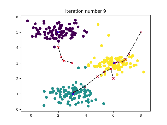
def plotProgresskMeans(X, centroids, previous, idx, K, i):
    # PLOTPROGRESSKMEANS is a helper function that displays the progress of
    # k-Means as it is running. It is intended for use only with 2D data.
    #   PLOTPROGRESSKMEANS(X, centroids, previous, idx, K, i) plots the data
    #   points with colors assigned to each centroid. With the previous
    #   centroids, it also plots a line between the previous locations and
    #   current locations of the centroids.
    #

    # Plot the examples
    plotDataPoints(X, idx, K)

    # Plot the centroids as black x's
    plt.plot(previous[:, 0], previous[:, 1], 'rx')
    plt.plot(centroids[:, 0], centroids[:, 1], 'bx')

    # Plot the history of the centroids with lines
    for j in range(size(centroids, 0)):
        # matplotlib can't draw line like [x1,y1] to [x2,y2]
        # it have to write like [x1,x2] to [y1,y2] f**k!
        plt.plot(r_[centroids[j, 0], previous[j, 0]],
                 r_[centroids[j, 1], previous[j, 1]], 'k--')

    # Title
    plt.title('Iteration number {}'.format(i))


def runkMeans(X: ndarray, initial_centroids: ndarray, max_iters: int,
              plot_progress=False):
    # RUNKMEANS runs the K-Means algorithm on data matrix X, where each row of X
    # is a single example
    #   [centroids, idx] = RUNKMEANS(X, initial_centroids, max_iters, ...
    #   plot_progress) runs the K-Means algorithm on data matrix X, where each
    #   row of X is a single example. It uses initial_centroids used as the
    #   initial centroids. max_iters specifies the total number of interactions
    #   of K-Means to execute. plot_progress is a true/false flag that
    #   indicates if the function should also plot its progress as the
    #   learning happens. This is set to false by default. runkMeans returns
    #   centroids, a Kxn matrix of the computed centroids and idx, a m x 1
    #   vector of centroid assignments (i.e. each entry in range [1..K])
    #

    # Plot the data if we are plotting progress
    if plot_progress:
        plt.figure()

    # Initialize values
    m, n = shape(X)
    K = size(initial_centroids, 0)
    centroids = initial_centroids.copy()
    previous_centroids = centroids.copy()
    idx = zeros((m, 1))

    # Run K-Means
    for i in range(max_iters):

        # Output progress
        print('K-Means iteration {}/{}...\n'.format(i, max_iters))

        # For each example in X, assign it to the closest centroid
        idx = findClosestCentroids(X, centroids)

        # Optionally, plot progress here
        if plot_progress:
            plotProgresskMeans(X, centroids, previous_centroids, idx, K, i)
            previous_centroids = centroids.copy()

        # Given the memberships, compute new centroids
        centroids = computeCentroids(X, idx, K)

    if plot_progress:
        plt.show()

    return centroids, idx


def kMeansInitCentroids(X: ndarray, K: int):
    # KMEANSINITCENTROIDS This function initializes K centroids that are to be
    # used in K-Means on the dataset X
    #   centroids = KMEANSINITCENTROIDS(X, K) returns K initial centroids to be
    #   used with the K-Means on the dataset X
    #

    # You should return this values correctly
    centroids = zeros((K, size(X, 1)))

    # ====================== YOUR CODE HERE ======================
    # Instructions: You should set centroids to randomly chosen examples from
    #               the dataset X
    #
    # Initialize the centroids to be random examples
    # Randomly reorder the indices of examples
    randidx = permutation(size(X, 0))
    # Take the first K examples as centroids
    centroids = X[randidx[:K, ], :]

    # =============================================================

    return centroids


def featureNormalize(X: ndarray):
    # FEATURENORMALIZE Normalizes the features in X
    #   FEATURENORMALIZE(X) returns a normalized version of X where
    #   the mean value of each feature is 0 and the standard deviation
    #   is 1. This is often a good preprocessing step to do when
    #   working with learning algorithms.

    mu = mean(X, axis=0)
    X_norm = X - mu

    sigma = std(X_norm, axis=0, ddof=1)
    X_norm /= sigma

    # ============================================================

    return X_norm, mu, sigma


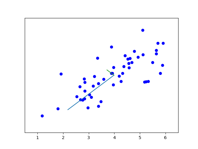
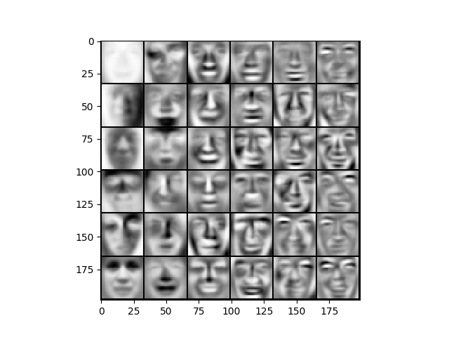
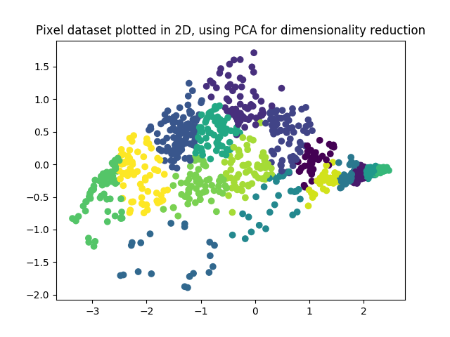
def pca(X: ndarray):
    # PCA Run principal component analysis on the dataset X
    #   [U, S, X] = pca(X) computes eigenvectors of the covariance matrix of X
    #   Returns the eigenvectors U, the eigenvalues (on diagonal) in S
    #

    # Useful values
    m, n = shape(X)

    # You need to return the following variables correctly.
    # U = zeros(n)
    # S = zeros(n)

    # ====================== YOUR CODE HERE ======================
    # Instructions: You should first compute the covariance matrix. Then, you
    #               should use the "svd" function to compute the eigenvectors
    #               and eigenvalues of the covariance matrix.
    #
    # Note: When computing the covariance matrix, remember to divide by m (the
    #       number of examples).
    #

    Sigma = X.T@ X/m
    U, S, V = svd(Sigma)

    # =========================================================================

    return U, diag(S)


def drawline(p1, p2, *arg):
    # DRAWLINE Draws a line from point p1 to point p2
    #   DRAWLINE(p1, p2) Draws a line from point p1 to point p2 and holds the
    #   current figure
    plt.plot(r_[p1[0], p2[0]], r_[p1[1], p2[1]], arg)


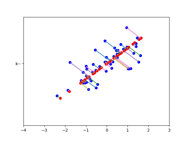
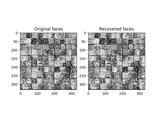
def projectData(X, U, K):
    # PROJECTDATA Computes the reduced data representation when projecting only
    # on to the top k eigenvectors
    #   Z = projectData(X, U, K) computes the projection of
    #   the normalized inputs X into the reduced dimensional space spanned by
    #   the first K columns of U. It returns the projected examples in Z.
    #

    # You need to return the following variables correctly.
    Z = zeros((size(X, 0), K))

    # ====================== YOUR CODE HERE ======================
    # Instructions: Compute the projection of the data using only the top K
    #               eigenvectors in U (first K columns).
    #               For the i-th example X(i,:), the projection on to the k-th
    #               eigenvector is given as follows:
    #                    x = X(i, :)';
    #                    projection_k = x' * U(:, k);
    #
    U_reduce = U[:, : K]
    Z = X @ U_reduce

    # =============================================================

    return Z


def recoverData(Z, U, K):
    # RECOVERDATA Recovers an approximation of the original data when using the
    # projected data
    #   X_rec = RECOVERDATA(Z, U, K) recovers an approximation the
    #   original data that has been reduced to K dimensions. It returns the
    #   approximate reconstruction in X_rec.
    #

    # You need to return the following variables correctly.
    X_rec = zeros((size(Z, 0), size(U, 0)))

    # ====================== YOUR CODE HERE ======================
    # Instructions: Compute the approximation of the data by projecting back
    #               onto the original space using the top K eigenvectors in U.
    #
    #               For the i-th example Z(i,:), the (approximate)
    #               recovered data for dimension j is given as follows:
    #                    v = Z(i, :)';
    #                    recovered_j = v' * U(j, 1:K)';
    #
    #               Notice that U(j, 1:K) is a row vector.
    #

    U_reduce = U[:, : K]

    X_rec = Z @ U_reduce.T

    # =============================================================

    return X_rec


def displayData(X: ndarray, e_width=0):
    if e_width == 0:
        e_width = int(round(sqrt(X.shape[1])))
    m, n = X.shape

    # 单独一个样本的像素大小
    e_height = int(n/e_width)

    # 分割线
    pad = 1

    # 整一副图的像素大小
    d_rows = int(floor(sqrt(m)))
    d_cols = int(ceil(m / d_rows))
    d_array = mat(
        ones((pad+d_rows*(e_height+pad), pad + d_cols * (e_width+pad))))

    curr_ex = 0
    for j in range(d_rows):
        for i in range(d_cols):
            if curr_ex > m:
                break
            max_val = max(abs(X[curr_ex, :]))
            d_array[pad+j*(e_height+pad) + 0:pad+j*(e_height+pad) + e_height,
                    pad+i*(e_width+pad)+0:pad+i*(e_width+pad) + e_width] = \
                X[curr_ex, :].reshape(e_height, e_width)/max_val
            curr_ex += 1
        if curr_ex > m:
            break
    # 转置一下放正
    plt.imshow(d_array.T, cmap='Greys')