EM算法与EM路由
搞定了yolo,终于可以学习点新的东西了。今天就学习一波胶囊网络中的EM路由。 先推荐一个课程资料,杜克大学的统计学课程,从python讲到c++,从矩阵计算讲到概率统计,从jit讲到cuda编程。看看人家本科生学的东西。。。
EM算法
詹森不等式
对于一个凸函数\(f\),\(E[f(x)]\geq f(E[x])\),将其反转获得一个凹函数。 如果一个函数\(f(x)\)在区间内都有\(f''(x)\geq 0\),那么它是一个凸函数。例如\(f(x)=log\ x\),\(f''(x)=-\frac{1}{x^2}\),说明他在\(x\in (0,+ \infty]\)是一个凸函数,詹森不等式的直观说明如下。
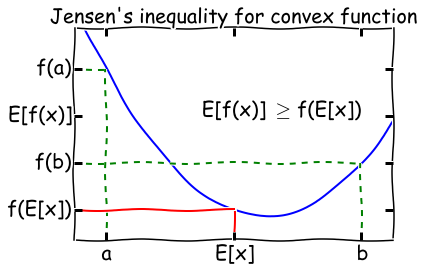
其实只有当\(f(x)\)为常数时,詹森不等式才会相等。
这里使用概率论表述的\(E\),其实际就是积分。也就是说先经过凸函数的期望值必然大于等于期望的凸函数值。
完整信息的最大似然
设置一个实验,硬币A向上的概率为\(\theta_A\)的,硬币B向上的概率为\(\theta_B\),接着一共做m此实验,每次实验随机选择一个硬币,投掷n次,并记录向下和向下的次数。如果我们记录了每个样本所使用的硬币,那我们就有完整的信息可以估计\(\theta_A\)和\(\theta_B\)。
假设我们做了5次实验,每次向上的次数记录成向量\(x\),并且使用的硬币顺序为\(A,A,B,A,B\)。他的似然函数为: \[ \begin{aligned} L(\theta_A,\theta_B)&= p(x_1; \theta_A)\cdot p(x_2; \theta_A)\cdot p(x_3; \theta_B) \cdot p(x_4; \theta_A) \cdot p(x_5; \theta_B) \\ &=B(n,\theta_A).pmf(x_1)\cdot B(n,\theta_A).pmf(x_2)\cdot B(n,\theta_B).pmf(x_3)\cdot B(n,\theta_A).pmf(x_4)\cdot B(n,\theta_B).pmf(x_5) \end{aligned} \] 其中二项分布的概率计算方式为: \[ \begin{aligned} \because X & \sim B(n,p)\\ \therefore P(X=k) &= \binom{n}{k} p^k (1-p)^{n-k} \\ &= C_n^k p^{k}(1-p)^{n-k} \end{aligned} \]
将似然函数对数化:
\[ \begin{aligned} L(\theta_A,\theta_B)=\log p(x_1; \theta_A) + \log p(x_2; \theta_A) +\log p(x_3; \theta_B) + \log p(x_4; \theta_A) +\log p(x_5; \theta_B) \end{aligned} \]
\(p(x_i; \theta)\)是二项式分布的概率质量函数,其中\(n=m,p=\theta\)。我们会使用\(z_i\)来表示第\(i\)个硬币的标签。
使用最小化函数求解似然
from numpy.core.umath_tests import matrix_multiply as mm |
可以发现似然估计的估计值相当近似与精确计算所得到的结论。
当信息缺失时的最大似然
当我们没有记录实验所使用的硬币种类时,这个问题的解决就开始困难起来了。有一种解决问题的方式就是我们根据这个样本是由\(A\)或\(B\)产生的来给每个样本假设权重\(\boldsymbol{w}_i\)。直觉上来想,权重应该是\(\boldsymbol{z}_i\)的后验分布: \[ \begin{aligned} w_i = p(z_i \ | \ x_i; \theta) \end{aligned} \]
假设我们有\(\theta\)的一些估计值,如果我们知道\(z_i\),那我们就可以估计出\(\theta\),因为我们相当于拥有了全部的似然信息。EM算法的基本思想就是先猜测\(\theta\),然后计算出\(z_i\),接着继续更新\(\theta\)再计算\(z_i\),重复数次直到收敛。
非书面的表述:首先考虑一个对数似然函数作为曲线(曲面),他的\(x\)轴表示\(\theta\)。找到另一个\(\theta\)的函数\(\boldsymbol{Q}\),他是对数似然函数的下界,在特定的\(\theta\)值时对数似然函数与函数\(\boldsymbol{Q}\)接触。接下来找到这个\(\theta\)的值,并且使函数\(\boldsymbol{Q}\)最大化,重复这个过程,是下界函数\(\boldsymbol{Q}\)和对数似然函数的最大值相同,那么我们就得到了最大对数似然~
从下图可以理解,每次迭代都能找到新的下界函数\(\boldsymbol{Q}\)和当前最大的对数似然,等到迭代到一定程度时,就找到了全局的最大的对数似然。
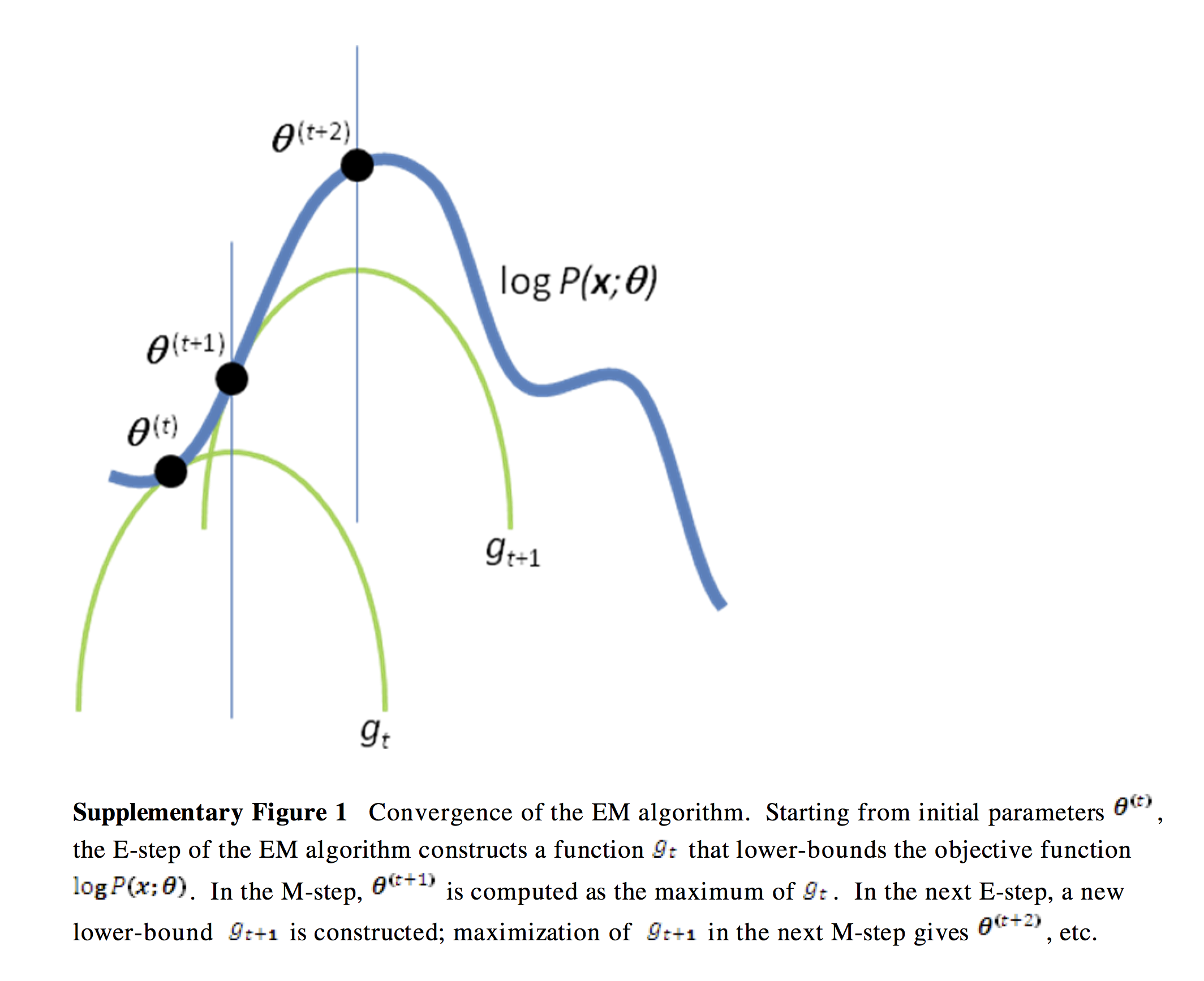
当然,还有个问题就是如何找到这个对数似然函数的下界函数\(\boldsymbol{Q}\),这就需要使用詹森不等式来进行数学推理。
推导
在EM算法的E-step中,我们确定一个函数,他是对数似然的下界。
\[
\begin{align}
l &= \sum_i{\log p(x_i; \theta)} && \text{定义对数似然函数}
\\
&= \sum_i \log \sum_{z_i}{p(x_i, z_i; \theta)} &&
\text{在函数中加入隐变量$z$} \\
&= \sum_i \log \sum_{z_i} Q_i(z_i) \frac{p(x_i, z_i;
\theta)}{Q_i(z_i)} && \text{贝叶斯定理得$Q_i$为$z_i$分布} \\
&= \sum_i \log E_{z_i}[\frac{p(x_i, z_i; \theta)}{Q_i(z_i)}]
&& \text{得到期望 - 就是EM中的E} \\
&\geq \sum E_{z_i}[\log \frac{p(x_i, z_i; \theta)}{Q_i(z_i)}]
&& \text{使用詹森不等式计算凹的对数似然函数} \\
&\geq \sum_i \sum_{z_i} Q_i(z_i) \log \frac{p(x_i, z_i;
\theta)}{Q_i(z_i)} && \text{得到期望的定义}
\end{align}
\]
我们如何确定分布\(\boldsymbol{Q_i}\)?我们想要\(\boldsymbol{Q}\)函数与对数似然函数进行接触,并且也知道了詹森不等式相等的充要条件就是这个函数为常数,因此:
\[ \begin{align} \frac{p(x_i, z_i; \theta)}{Q_i(z_i)} =& c \\ \implies Q_i(z_i) &\propto p(x_i, z_i; \theta)\\ \implies Q_i(z_i) &= \frac{p(x_i, z_i; \theta) }{\sum_{z_i}{p(x_i, z_i; \theta) } } &&\text{因为 $\boldsymbol{Q}$ 是个分布且和为1} \\ \implies Q_i(z_i) &= \frac{p(x_i, z_i; \theta) }{ {p(x_i, \theta) } } && \text{边缘化 $z_i$}\\ \implies Q_i(z_i) &= p(z_i | x_i; \theta) && \text{根据条件概率定义} \end{align} \]
因此得到\(\boldsymbol{Q_i}\)就是\(z_i\)的后验概率,这就完成了E-step。
在M-step中,我找到最大化对数似然函数下界时的\(\theta\)值,然后我们迭代E和M即可。
所以EM算法是在缺少信息的情况下最大化似然的优化算法,或者说他可以很方便的添加隐变量来简化最大似然计算。
例子
现在如果我们忘记记录了投掷硬币的顺序,那我们来求解一波A、B硬币向上的概率。
对于E-step,我们:
\[ \begin{align} w_j &= Q_i(z_i = j) \\ &= p(z_i = j \mid x_i; \theta) \\ &= \frac{p(x_i \mid z_i = j; \theta) p(z_i = j; \phi)} {\sum_{l=1}^k{p(x_i \mid z_i = l; \theta) p(z_i = l; \phi) } } && \text{贝叶斯准则} \\ &= \frac{\theta_j^h(1-\theta_j)^{n-h} \phi_j}{\sum_{l=1}^k \theta_l^h(1-\theta_l)^{n-h} \phi_l} && \text{代入二项分布公式} \\ &= \frac{\theta_j^h(1-\theta_j)^{n-h} }{\sum_{l=1}^k \theta_l^h(1-\theta_l)^{n-h} } && \text{为了简单起见使 $\phi$ 为常数} \end{align} \]
对于M-step,我们需要找到最大时的\(\theta\)值。
\[ \begin{align} & \sum_i \sum_{z_i} Q_i(z_i) \log \frac{p(x_i, z_i; \theta)}{Q_i(z_i)} \\ &= \sum_{i=1}^m \sum_{j=1}^k w_j \log \frac{p(x_i \mid z_i=j; \theta) \, p(z_i = j; \phi)}{w_j} \\ &= \sum_{i=1}^m \sum_{j=1}^k w_j \log \frac{\theta_j^h(1-\theta_j)^{n-h} \phi_j}{w_j} \\ &= \sum_{i=1}^m \sum_{j=1}^k w_j \left( h \log \theta_j + (n-h) \log (1-\theta_j) + \log \phi_j - \log w_j \right) \end{align} \]
我们使用区间的方式解决\(\theta_s\)导数消失的问题: \[ \begin{align} \sum_{i=1}^m w_s \left( \frac{h}{\theta_s} - \frac{n-h}{1-\theta_s} \right) &= 0 \\ \implies \theta_s &= \frac {\sum_{i=1}^m w_s h}{\sum_{i=1}^m w_s n} \end{align} \]
第一种直接的代码
xs = np.array([(5, 5), (9, 1), (8, 2), (4, 6), (7, 3)]) |
结果
Iteration: 1 |
NOTE: 他这里的对数似然函数是根据上面的公式推导之后简化而来的,所以直接对\(\theta\)做对数即可,下面我按最基本的思路来写了一个例程。
我的代码
n = 10 # 实验次数 |
结果
Iteration: 1 |
NOTE: 就是对数似然值和例程计算的不一样。。
混合模型
从一个简单的混合模型开始,即k-means,k-means不使用EM算法,但是可以结合EM算法帮助理解EM算法如何用于高斯混合模型。
K-means
这个算法比较简单,初始化选择\(k\)个中心点,然后做如下:
- 找到每个点与中心点的距离
- 给每个点分配最近的中心点
- 根据所分配的点来更新中心点位置
下面给出一段程序示例:
from numpy.core.umath_tests import inner1d |
结果
高斯混合模型
\(k\)个高斯分布混合具有以下的概率密度函数: \[ \begin{align} p(x) = \sum_{j=1}^k \pi_j \phi(x; \mu_j, \sigma_j) \end{align} \]
\(\pi_j\)是第\(j\)个高斯分布的权重,且:
\[ \begin{align} \phi(x; \mu, \sigma) = \frac{1}{(2 \pi)^{d/2}|\sigma|^{1/2 } } \exp \left( -\frac{1}{2}(x-\mu)^T\sigma^{-1}(x-\mu) \right) \end{align} \]
假设我们观察\(y_1, y2, \ldots, y_n\)作为来自高斯混合模型的样本,那么对数似然为: \[ \begin{align} l(\theta) = \sum_{i=1}^n \log \left( \sum_{j=1}^k \pi_j \phi(y_i; \mu_j, \sigma_j) \right) \end{align} \]
其中\(\theta = (\pi, \mu, \sigma)\),很难拟合这种对数似然最大值的参数,因为他们要在对数函数中求和。
使用EM算法
假设我们增加潜在变量\(z\),它表明我们观察到的\(y\)来自于第\(k\)个高斯分布。其中E-step和M-step的推导与之前的例子类似,只是变量更多。
在E-step我们想要计算样本\(x_i\)输入第\(j\)个类别的后验概率,给定参数\(\theta =(\pi,\mu,\sigma)\)
NOTE: 这里后验概率有的地方使用公式\(p(j|x_i)\),这里使用\(w_j^i\)来表示。
\[ \begin{align} w_j^i &= Q_i(z^i = j) \\ &= p(z^i = j \mid y^i; \theta) \\ &= \frac{p(x^i \mid z^i = j; \mu, \sigma) p(z^i = j; \pi)} {\sum_{l=1}^k{p(y^i \mid z^i = l; \mu, \sigma) p(z^i = l; \pi) } } && \text{贝叶斯定理} \\ &= \frac{\phi(x^i; \mu_j, \sigma_j) \pi_j}{\sum_{l=1}^k \phi(x^i; \mu_l, \sigma_l) \pi_l} \end{align} \]
在M-step中,我们要找到\(\theta
= (w, \mu, \sigma)\)来最大化\(\boldsymbol{Q}\)函数,对应与真实对数似然函数的下界。
\[ \begin{align} \sum_{i=1}^{m}\sum_{j=1}^{k} Q(z^i=j) \log \frac{p(x^i \mid z^i= j; \mu, \sigma) p(z^i=j; \pi)}{Q(z^i=j)} \end{align} \]
通过分别取\((w, \mu, \sigma)\)的导数并求解(使用拉格朗日乘数构造约束\(\sum_{j=1}^k w_j = 1\)来求解),我们得到:
\[ \begin{align} \pi_j &= \frac{1}{m} \sum_{i=1}^{m} w_j^i \\ \mu_j &= \frac{\sum_{i=1}^{m} w_j^i x^i}{\sum_{i=1}^{m} w_j^i} \\ \sigma_j &= \frac{\sum_{i=1}^{m} w_j^i (x^i - \mu)(x^i - \mu)^T}{\sum_{i1}^{m} w_j^i} \end{align} \]
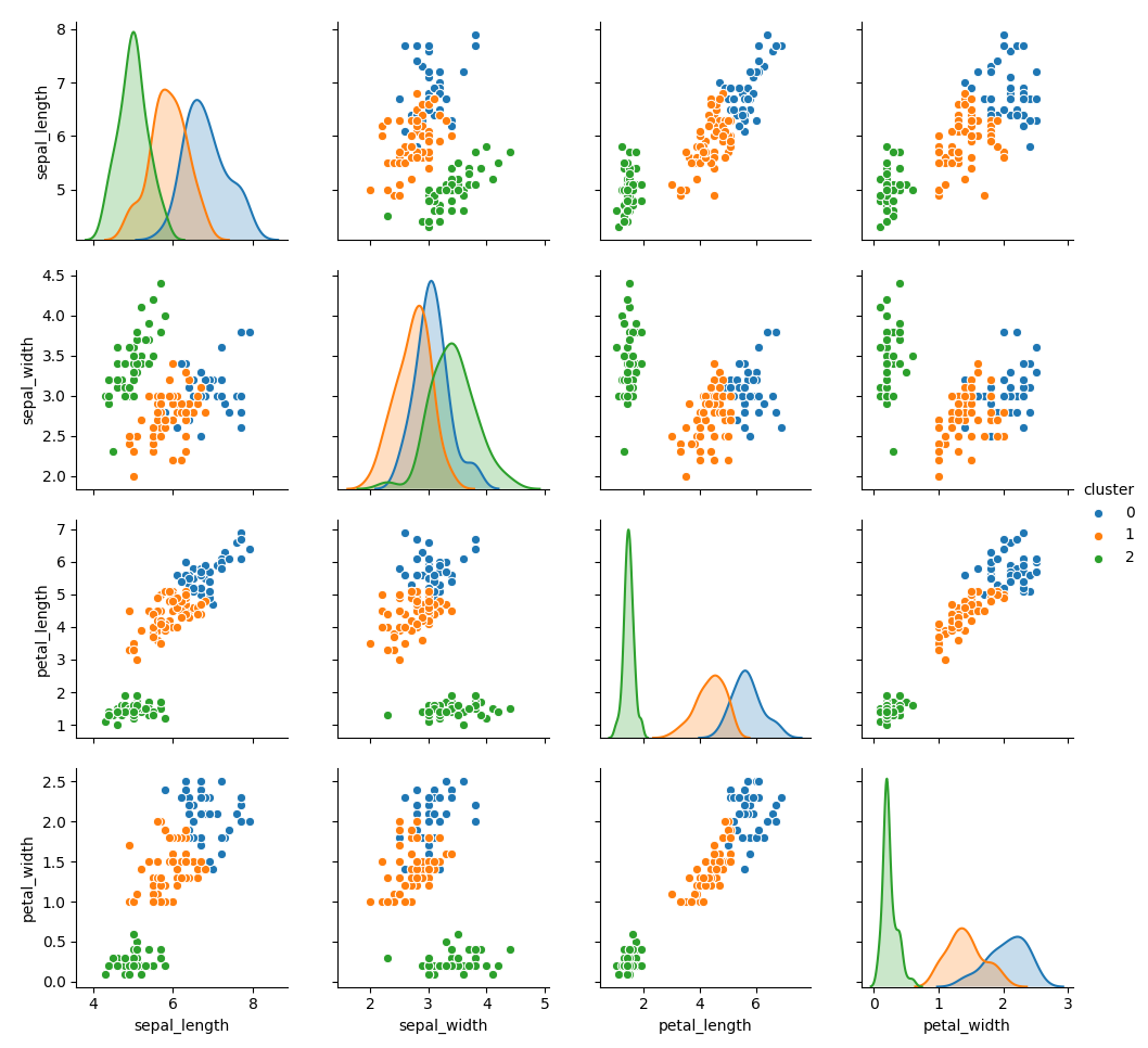
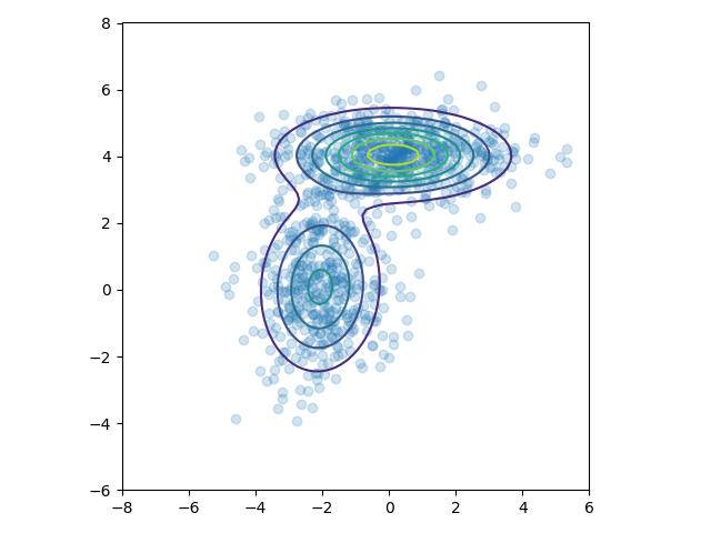
代码
from scipy.stats import multivariate_normal |
结果
胶囊网络
矩阵胶囊
现在的矩阵胶囊与之前的胶囊不是很一样了,因为胶囊是矩阵,就不能把模长作为激活了。所以多加一个标量\(a\)来表示激活值。
矩阵胶囊的主体,名字也变了一下,叫做姿态矩阵,这里是\(4\times4\)的矩阵。

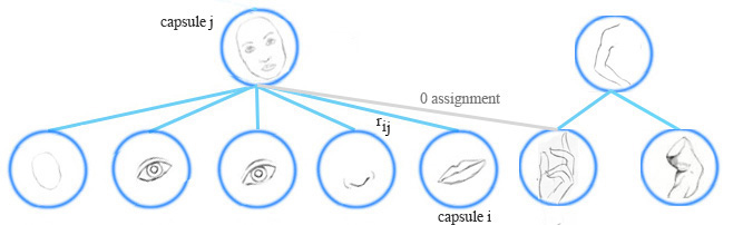
胶囊投票机制
在胶囊网络中,通过寻找底层胶囊投票之间的一致性来检测一个高层特征(比如一张脸),对于来自胶囊\(i\)对父胶囊\(j\)的投票\(\boldsymbol{V}_{ij}\),通过将胶囊\(i\)的姿态矩阵\(\boldsymbol{P}_i\)和视角不变矩阵\(W_{ij}\)相乘得到。
\[ \begin{split} &\boldsymbol{V}_{ij} =\boldsymbol{P}_i W_{ij} \quad \end{split} \]
基于投票\(\boldsymbol{V}_{ij}\)和其他投票\((\boldsymbol{V}_{o_{1}j} \ldots \boldsymbol{V}_{o_{k}j})\)相似度来计算胶囊\(i\)被分组到胶囊\(j\)中的概率。
胶囊分配
EM算法对低层的胶囊进行聚类,也计算底层胶囊与上层胶囊间分配概率\(r_{ij}\)。例如一个表示手的胶囊不属于脸的胶囊,他们的分配概率就被抑止到0,\(r_{ij}\)也受到胶囊激活的影响。
计算胶囊激活和姿态矩阵
在EM聚类中,我们将数据使用正态分布来表现。在EM路由中,我们也对父胶囊使用正态分布来建模,姿态矩阵\(M\)是\(4\times4\)的矩阵,即16个分量。我们对姿态矩阵建立16个\(\mu\),16个\(\sigma\)的高斯分布,每个\(\mu\)就表征了姿态矩阵的每个分量。注意为了避免在概率密度函数中求逆,胶囊网络中的\(\sigma\)是被固定成一个对角矩阵的。
让\(v_{ij}\)作为底层胶囊\(i\)对父胶囊\(j\)的投票,\(v^{n}_{ij}\)代表着第n个分量。我们使用高斯概率密度函数
\[ \begin{split} P(x) & = \frac{1}{\sigma \sqrt{2\pi } }e^{-(x - \mu)^{2}/2\sigma^{2} } \\ \end{split} \]
来计算属于胶囊\(j\)正态分布的投票\(v^{n}_{ij}\)概率。 \[ \begin{split} p^n_{i \vert j} & = \frac{1}{\sqrt{2 \pi ({\sigma^n_j})^2 } } \exp{(- \frac{(v^n_{ij}-\mu^n_j)^2}{2 ({\sigma^n_j})^2})} \\ \end{split} \]
取其对数:
\[ \begin{split} \ln(p^n_{i \vert j}) &= \ln \frac{1}{\sqrt{2 \pi ({\sigma^n_j})^2 } } \exp{(- \frac{(v^n_{ij}-\mu^n_j)^2}{2 ({\sigma^n_j})^2})} \\ \\ &= - \ln(\sigma^n_j) - \frac{\ln(2 \pi)}{2} - \frac{(v^n_{ij}-\mu^n_j)^2}{2 ({\sigma^n_j})^2}\\ \end{split} \]
接下来估计胶囊激活的损失值,越低的损失值,代表胶囊越有可能被激活。如果损失值较大,就代表投票与父胶囊的高斯分布不匹配,因此激活概率较小。
让\(cost_{ij}\)作为胶囊\(i\)激活胶囊\(j\)的损失,是负的对数似然也可以称之为熵(熵越小,那就意味似然估计越准): \[ cost^n_{ij} = - \ln(P^n_{i \vert j}) \]
由于胶囊\(i\)与胶囊\(j\)之间的联系并不相同,因此我们将在运行时按比例\(r_{ij}\)来分配\(cost\),那下层胶囊的\(cost\)计算为:
\[ \begin{split} cost^n_j &= \sum_i r_{ij} cost^n_{ij} \\ &= \sum_i - r_{ij} \ln(p^n_{i \vert j}) \\ &= \sum_i r_{ij} \big( \frac{(v^n_{ij}-\mu^n_j)^2}{2 ({\sigma^n_j})^2} + \ln(\sigma^n_j) + \frac{\ln(2 \pi)}{2} \big)\\ &= \frac{\sum_i r_{ij} (\sigma^n_j)^2}{2 (\sigma^n_j)^2} + (\ln(\sigma^n_j) + \frac{\ln(2 \pi)}{2}) \sum_i r_{ij} \\ &= \big(\ln(\sigma^n_j) + \beta_v \big) \sum_i r_{ij} \quad \beta_v\text{是待优化参数} \end{split} \]
有了\(cost\)值,使用\(a_j\)来决定胶囊\(j\)是否被激活: \[ a_j = sigmoid(\lambda(\beta_a - \sum_h cost^n_j)) \]
这里面的\(\beta_a,\beta_v\)是根据反向传播进行优化的,所以并不需要直接计算。
其中的\(r_{ij},\mu,\sigma,a_j\)是根据EM路由来计算的。\(\lambda\)是根据温度参数\(\frac{1}{temperature}\)来计算(退火策略),随着\(r_{ij}\)越来越好,就降低temperature以获得更大的\(\lambda\),也就是增加\(sigmoid\)的陡度,这样就更加在更加小的范围内微调\(r_{ij}\)。
EM路由
这一块是重点,所以我要仔细看每个公式细节。并且要一步一步的渐进的看。
新动态路由1
首先用一个矩阵\(\boldsymbol{P}_{i}, i=1,\ldots,n\)来表示第\(l\)层的胶囊,用矩阵\(\boldsymbol{M}_j, j=1,\ldots,k\)来表示第\(l+1\)层的胶囊。在做EM路由的过程中,他将\(P_i\)变成长16的向量,且协方差矩阵为对角阵。
\[ \begin{aligned} &p_{ij} \leftarrow N(\boldsymbol{P}_i;\boldsymbol{\mu}_j,\boldsymbol{\sigma}^2_j) && \text{计算概率密度} \\ &R_{ij} \leftarrow \frac{\pi_j p_{ij} }{\sum\limits_{j=1}^k\pi_j p_{ij} } && \text{计算后验概率} \\ &r_{ij}\leftarrow \frac{R_{ij } }{\sum\limits_{i=1}^n R_{ij } } && \text{计算归一化后验概率} \\ &\boldsymbol{M}_j \leftarrow \sum\limits_{i=1}^n r_{ij}\boldsymbol{P}_i && \text{计算新样本} \\ &\boldsymbol{\sigma}^2_j \leftarrow \sum\limits_{i=1}^n r_{ij}(\boldsymbol{P}_i-\boldsymbol{M}_j)^2 && \text{更新}\sigma \\ &\pi_j \leftarrow \frac{1}{n}\sum\limits_{i=1}^n R_{ij} && \text{更新聚类中心}\pi \end{aligned} \]
这里的\(R_{ij}\)就是后验概率,也就是在EM算法中使用的\(w_j\)。
新动态路由2
前面讲道理有一个激活标量\(a_j\)来衡量胶囊单元的显著程度,根据EM算法计算我们可以得到\(\pi_j\)为第\(l+1\)层胶囊的聚类中心,但我们不能选择\(\pi\)因为:
- \(\pi_j\)是归一化的,就是我们只想得到他的显著程度,而不是显著程度的概率。
- \(\pi_j\)不能反映出类内的元素特征是否相似。
现在再看前面所使用的激活标量\(a_j\),他既考虑了似然估计值\(cost_j^h\),又考虑了显著程度\(\pi_j\)。所以作者直接将\(a_j\)替换了\(\pi_j\),这样虽然不完全与原始EM算法相同,但是也能收敛,得到新的动态路由:
\[ \begin{aligned} &p_{ij} \leftarrow N(\boldsymbol{P}_i;\boldsymbol{\mu}_j,\boldsymbol{\sigma}^2_j) && \text{计算概率密度} \\ &R_{ij} \leftarrow \frac{a_j p_{ij} }{\sum\limits_{j=1}^k a_j p_{ij} } && \text{计算后验概率} \\ &r_{ij}\leftarrow \frac{R_{ij } }{\sum\limits_{i=1}^n R_{ij } } && \text{归一化后验概率} \\ &\boldsymbol{M}_j \leftarrow \sum\limits_{i=1}^n r_{ij}\boldsymbol{P}_i && \text{计算新样本} \\ &\boldsymbol{\sigma}^2_j \leftarrow \sum\limits_{i=1}^n r_{ij}(\boldsymbol{P}_i-\boldsymbol{M}_j)^2 && \text{更新}\sigma \\ & cost_j \leftarrow \left(\beta_v+\sum\limits_{l=1}^d \ln \boldsymbol{\sigma}_j^l \right)\sum\limits_i r_{ij} && \text{计算熵} \\ & a_j \leftarrow sigmoid(\lambda(\beta_a - \sum_h cost^h_j)) && \text{更新}a_j \end{aligned} \]
新动态路由3
上面好像没什么问题。但是没有使用底层胶囊的激活值\(a^{last}_i\),作者在计算归一化后验概率\(r_{ij}\leftarrow \frac{R_{ij } }{\sum\limits_{i=1}^n R_{ij } }\)的时候加入:
\[ \begin{aligned} &p_{ij} \leftarrow N(\boldsymbol{P}_i;\boldsymbol{\mu}_j,\boldsymbol{\sigma}^2_j) && \text{计算概率密度} \\ &R_{ij} \leftarrow \frac{a_j p_{ij} }{\sum\limits_{j=1}^k a_j p_{ij} } && \text{计算后验概率} \\ &r_{ij}\leftarrow \frac{a_i^{last}R_{ij } }{\sum\limits_{i=1}^n a_i^{last} R_{ij } } && \text{计算归一化后验概率} \\ &\boldsymbol{M}_j \leftarrow \sum\limits_{i=1}^n r_{ij}\boldsymbol{P}_i && \text{计算新样本} \\ &\boldsymbol{\sigma}^2_j \leftarrow \sum\limits_{i=1}^n r_{ij}(\boldsymbol{P}_i-\boldsymbol{M}_j)^2 && \text{更新}\sigma \\ & cost_j \leftarrow \left(\beta_v+\sum\limits_{l=1}^d \ln \boldsymbol{\sigma}_j^l \right)\sum\limits_i r_{ij} && \text{计算熵} \\ & a_j \leftarrow sigmoid(\lambda(\beta_a - \sum_h cost^h_j)) && \text{更新}a_j \end{aligned} \]
新动态路由4
因为\(\sum\limits_i r_{ij}=1\),所以下面还可以化简。
\[ \begin{aligned} &p_{ij} \leftarrow N(\boldsymbol{P}_i;\boldsymbol{\mu}_j,\boldsymbol{\sigma}^2_j) && \text{计算概率密度} \\ &R_{ij} \leftarrow \frac{a_j p_{ij} }{\sum\limits_{j=1}^k a_j p_{ij} } && \text{计算后验概率} \\ &r_{ij}\leftarrow \frac{a_i^{last}R_{ij } }{\sum\limits_{i=1}^n a_i^{last} R_{ij } } && \text{计算归一化后验概率} \\ &\boldsymbol{M}_j \leftarrow \sum\limits_{i=1}^n r_{ij}\boldsymbol{P}_i && \text{计算新样本} \\ &\boldsymbol{\sigma}^2_j \leftarrow \sum\limits_{i=1}^n r_{ij}(\boldsymbol{P}_i-\boldsymbol{M}_j)^2 && \text{更新}\sigma \\ & cost_j \leftarrow \left(\beta_v+\sum\limits_{l=1}^d \ln \boldsymbol{\sigma}_j^l \right)\sum\limits_i a_i^{last} R_{ij} && \text{计算熵} \\ & a_j \leftarrow sigmoid(\lambda(\beta_a - \sum_h cost^h_j)) && \text{更新}a_j \end{aligned} \]
最终的动态路由
现在再把投票机制与视角不变矩阵加入进来,投票矩阵与上面描述一样\(\boldsymbol{V}_{ij}=\boldsymbol{P}_{i}\boldsymbol{W}_{ij}\)。
\[ \begin{aligned} &p_{ij} \leftarrow N(\boldsymbol{V}_{ij};\boldsymbol{\mu}_j,\boldsymbol{\sigma}^2_j) && \text{计算概率密度} \\ &R_{ij} \leftarrow \frac{a_j p_{ij} }{\sum\limits_{j=1}^k a_j p_{ij} } && \text{计算后验概率} \\ &r_{ij}\leftarrow \frac{a_i^{last}R_{ij } }{\sum\limits_{i=1}^n a_i^{last} R_{ij } } && \text{计算归一化后验概率} \\ &\boldsymbol{M}_j \leftarrow \sum\limits_{i=1}^n r_{ij}\boldsymbol{V}_{ij} && \text{计算新样本} \\ &\boldsymbol{\sigma}^2_j \leftarrow \sum\limits_{i=1}^n r_{ij}(\boldsymbol{V}_{ij}-\boldsymbol{M}_j)^2 && \text{更新}\sigma \\ & cost_j \leftarrow \left(\beta_v+\sum\limits_{l=1}^d \ln \boldsymbol{\sigma}_j^l \right)\sum\limits_i a_i^{last} R_{ij} && \text{计算熵} \\ & a_j \leftarrow sigmoid(\lambda(\beta_a - \sum_h cost^h_j)) && \text{更新}a_j \end{aligned} \]
代码
论文中的伪代码
官方的EM路由的顺序是和之前使用的EM算法不一样的,他先做M-step再做E-step,因为一开始我们是不知道父胶囊的分布,所以我们没有办法通过概率密度函数来计算后验分布,他这里比较简单粗暴,直接先把后验概率\(R_{ij}\)分配为1,再来算分配权重矩阵\(r_{ij}\)。 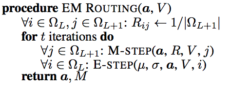
在M-step中计算出父胶囊正态分布的\(\mu,\sigma\)。然后计算熵\(cost\),再计算激活。
NOTE: 在论文或者tensorflow里面,\(log\)默认都是以\(e\)为底的。并且这里的h就是我上面用的n

在E-step中,我们有了之前的父胶囊的\(\mu,\sigma\),那我们根据正态分布公式计算概率密度\(p_{ij}\),然后贝叶斯公式更新后验概率\(R_{ij}\)。这样一个循环就形成了。 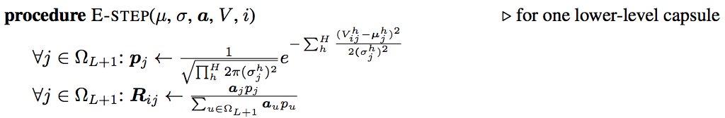
python实现
使用Tensorflow 1.14直接运行即可。主要就是看EM算法的实现部分,当然这里在计算\(a_j\)的时候,用的是迂回的方式来计算,避免值溢出。我再尝试过这个算法之后,感觉真的不咋地,思路很高深,但是效果没有那些简单粗暴的算法好,我还是喜欢谷歌提出一些网络,虽然没那么多数学原理,但是很直接有效。不过这个笔记对我拿来写论文还是很有帮助的。
import numpy as np |