半监督学习：MixMatch

第七个算法MixMatch: A Holistic Approach toSemi-Supervised Learning。此算法将之前的各个半监督学习算法进行融合，统一了主流方法，得到了最优的效果。此算法好，就是训练的过程慢一些。

算法理论

半监督学习主要以未标记数据减轻对标记数据的要求，许多半监督学习方法都是添加根据无标签数据所产生的损失，从而使得模型更好的将未知标签数据分类。在最近的算法中，所添加的大部分损失属于以下三类之一，首先设置一个模型\(\text{P}_{model}(y|x\theta)\)，可以从通过参数\(\theta\)从输入\(x\)中得到类别\(y\)。

1. 熵最小化

   代表,Pseudo-label: The simple and efficient semi-supervised learning method fordeep neural networks)。做法是鼓励模型输出无标签数据的标签。

   在许多半监督学习方法中，一个常见的基本假设是分类器的决策边界不应通过边缘数据分布的高密度区域。强制执行此操作的一种方法是要求分类器对未标记的数据输出低熵预测。如论文(Semi-supervised learning by entropy minimization)使用这种这种损失函数使得\(\text{P}_{model}(y|x\theta)\)关于无标签数据\(x\)的熵最小，这种方法和VAT结合可以得到更强的效果。pseudo label通过对无标签数据的高置信度预测构造出伪标签进行训练，从而隐式的最小化熵。MixMatch通过在无标签数据的预测分布上使用sharpening函数，也隐式的最小化熵。

2. 一致性正则

   鼓励模型在其输入受到扰动时产生相同的输出分布。最简单的例子如下，对于无标签数据\(x\)： \[ \begin{align} \| \text { Pmodel }(y | \text { Augment }(x) ; \theta)-\text { Pmodel }(y | \text { Augment }(x) ; \theta) \|_{2}^{2} \end{align}\tag{1} \] 注意\(\text { Augment }\)是随机变化，所以公式1中的两项是不一样的。mean teacher通过代替公式1中的一项，使用模型参数的滑动平均进行模型输出，这提供了一个更稳定的输出分布，并发现了过去经验可以改善当前结果。这些方法的缺点是它们使用特定于域的数据增强策略。VAT则通过计算扰动来解决这个问题，将这个扰动添加到输入中，从而最大程度的改变输出类别的分布。MixMatch则通过对图像进行标准的数据增强来添加一致性正则。

3. 一般正则化

   传统正则算法鼓励模型得到更好的拟合与泛化效果。在MixMatch中对模型参数用l2正则，同时数据增强使用mixup。

MixMatch就是一种集合上以上三种方法的新方法。总之，MixMatch引入了针对无标签数据的统一的损失项，既可以减少熵又可以保持一致正则性，还与一般正则化方法兼容。

MixMatch

首先给出一系列符号。给定一个batch的标记数据\(\mathcal{X}\)以及one-hot标签，一个batch的无标签数据\(\mathcal{U}\)，通过数据增强得到\(\mathcal{X}',\mathcal{U}'\)，然后对他们分别计算损失，最终整合所有损失：

\[ \begin{align} \mathcal{X}^{\prime}, \mathcal{U}^{\prime}=\operatorname{MixMatch}(\mathcal{X}, \mathcal{U}, T, K, \alpha) \end{align}\tag{2} \]

\[ \begin{align} \mathcal{L}_{\mathcal{X}}=\frac{1}{\left|\mathcal{X}^{\prime}\right|} \sum_{x, p \in \mathcal{X}^{\prime}} \mathrm{H}\left(p, \mathrm{p}_{\text {model }}(y | x ; \theta)\right) \end{align}\tag{3} \]

\[ \begin{align} \mathcal{L}_{\mathcal{U}}=\frac{1}{L\left|\mathcal{U}^{\prime}\right|} \sum_{u, q \in \mathcal{U}^{\prime}}\left\|q-\mathrm{p}_{\text {model }}(y | u ; \theta)\right\|_{2}^{2} \end{align}\tag{4} \]

\[ \begin{align} \mathcal{L}=\mathcal{L}_{\mathcal{X}}+\lambda_{\mathcal{U}} \mathcal{L}_{\mathcal{U}} \end{align}\tag{5} \]

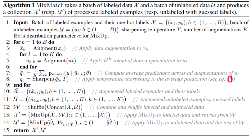
其中\(H(p,q)\)是分布\(p\)和\(q\)间的交叉熵，\(T,K,\alpha,\lambda_{\mathcal{U}}\)是超参数。完整的MixMatch如算法1所示。

现在来描述各个部分：

1. 数据增强

   对于一个batch\(\mathcal{X}\)中的每一个\(x_b\)，通过变化得到\(\hat{x}_{b}=\text { Augment }\left(x_{b}\right)\)(算法1第3行)。对于每个无标签数据\(u_b\)，我们生成\(K\)个增强\(\hat{u}_{b, k}=\text { Augment }\left(u_{b}\right), k \in(1, \ldots, K)\)(算法1第5行)。再使用每个\(u_b\)送入模型得到对应的猜测标签\(q_b\)。

2. 标签猜测

   有了猜测标签，我们将它用在无监督损失中，平均对\(u_b\)做\(K\)个增强的模型预测输出分布：

   \[ \begin{align} \bar{q}_{b}=\frac{1}{K} \sum_{k=1}^{K} \operatorname{Prodel}\left(y | \hat{u}_{b, k} ; \theta\right) \end{align}\tag{6} \]

   sharpening： 为了达到对熵最小化的目的，我们需要对给定数据增强预测的平均值\(\bar{q}_{b}\)进行sharpening，通过sharpening函数减小标签的分布熵。在代码中，是调整分类分布的温度系数：

   \[ \begin{align} \text { Sharpen }(p, T)_{i}:=p_{i}^{\frac{1}{T}} / \sum_{j=1}^{L} p_{j}^{\frac{1}{T}} \end{align}\tag{7} \]

   其中\(p\)是一些输入分类分布(在此算法中为\(\bar{q}_{b}\))，\(T\)是超参数。当\(T\rightarrow0\)，\(\text{Sharpen}(p,T)\)的输出会趋近于Dirac(one-hot)分布，降低温度系数会鼓励模型产生较低熵的预测。

3. mixup

   要应用mixup，我们首先需要将所有的带标签的增强数据和所有无标签样本以及对应的猜测标签收集起来(算法1第10-11行): \[ \begin{align} \hat{\mathcal{X}}=\left(\left(\hat{x}_{b}, p_{b}\right) ; b \in(1, \ldots, B)\right) \end{align}\tag{12} \] \[ \begin{align} \hat{\mathcal{U}}=\left(\left(\hat{u}_{b, k}, q_{b}\right) ; b \in(1, \ldots, B), k \in(1, \ldots, K)\right) \end{align}\tag{13} \]

   然后我们联合以上分布并进行混洗得到新的数据集\(\mathcal{W}\)作为mixup的输入，对每第\(i\)个样本对\(\hat{\mathcal{X}}\)，我们计算\(\operatorname{MixUp}\left(\hat{\mathcal{X}}_{i}, \mathcal{W}_{i}\right)\)并将结果添加到\(\mathcal{X}'\)(算法1第13行)，对于\(i\in(1,\ldots,|\bar{\mathcal{U}}|)\)我们计算\(\mathcal{U}_{i}^{\prime}=\operatorname{MixUp}\left(\hat{\mathcal{U}}_{i}, \mathcal{W}_{i+|\hat{\mathcal{X}}|}\right)\) for \(i \in(1, \ldots,|\hat{\mathcal{U}}|)\)。在这个过程中，带标签数据可能会和无标签数据产生混合。

4. 损失函数

   损失即标签数据的交叉熵结合无标签数据的差异性损失。

5. 超参数

   因为MixMatch结合了很多算法，所以超参数也特别的多，一般固定\(T=0.5，K=2\)，然后\(\alpha=0.75,\lambda_{\mathcal{U}}=100\)

消融测试结果：

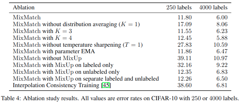
可以发现关键提升点在于锐化以及无标签数据间的mixup

代码

def distribution_summary(self, p_data, p_model, p_target=None):
    def kl(p, q):
        p /= tf.reduce_sum(p)
        q /= tf.reduce_sum(q)
        return -tf.reduce_sum(p * tf.log(q / p))

    tf.summary.scalar('metrics/kld', kl(p_data, p_model))
    if p_target is not None:
        tf.summary.scalar('metrics/kld_target', kl(p_data, p_target))

    for i in range(self.nclass):
        tf.summary.scalar('matching/class%d_ratio' % i, p_model[i] / p_data[i])
    for i in range(self.nclass):
        tf.summary.scalar('matching/val%d' % i, p_model[i])

def augment(self, x, l, beta, **kwargs):
    assert 0, 'Do not call.'

def guess_label(self, y, classifier, T, **kwargs):
    del kwargs
    logits_y = [classifier(yi, training=True) for yi in y]
    logits_y = tf.concat(logits_y, 0)
    # Compute predicted probability distribution py.
    # p_model_y shape = [K,batch,calss_num]
    p_model_y = tf.reshape(tf.nn.softmax(logits_y), [len(y), -1, self.nclass])
    # 求均值
    p_model_y = tf.reduce_mean(p_model_y, axis=0)
    # 锐化
    p_target = tf.pow(p_model_y, 1. / T)
    p_target /= tf.reduce_sum(p_target, axis=1, keep_dims=True)
    return EasyDict(p_target=p_target, p_model=p_model_y)

def model(self, batch, lr, wd, ema, beta, w_match, warmup_kimg=1024, nu=2, mixmode='xxy.yxy', dbuf=128, **kwargs):
    hwc = [self.dataset.height, self.dataset.width, self.dataset.colors]
    xt_in = tf.placeholder(tf.float32, [batch] + hwc, 'xt')  # For training
    x_in = tf.placeholder(tf.float32, [None] + hwc, 'x')
    y_in = tf.placeholder(tf.float32, [batch, nu] + hwc, 'y')
    l_in = tf.placeholder(tf.int32, [batch], 'labels')

    w_match *= tf.clip_by_value(tf.cast(self.step, tf.float32) / (warmup_kimg << 10), 0, 1)
    lrate = tf.clip_by_value(tf.to_float(self.step) / (FLAGS.train_kimg << 10), 0, 1)
    lr *= tf.cos(lrate * (7 * np.pi) / (2 * 8))
    tf.summary.scalar('monitors/lr', lr)
    # 设置mixup的模式，默认是标记数据会与(标记数据，无标记数据)混合，无标记数据会与(标记数据，无标记数据)混合
    augment = MixMode(mixmode)
    classifier = lambda x, **kw: self.classifier(x, **kw, **kwargs).logits

    # Moving average of the current estimated label distribution
    p_model = layers.PMovingAverage('p_model', self.nclass, dbuf)
    p_target = layers.PMovingAverage('p_target', self.nclass, dbuf)  # Rectified distribution (only for plotting)

    # Known (or inferred) true unlabeled distribution
    p_data = layers.PData(self.dataset)
    # K个增强就有K个无标签输入
    y = tf.reshape(tf.transpose(y_in, [1, 0, 2, 3, 4]), [-1] + hwc)
    # 得到锐化后的猜测标签以及原始猜测标签
    guess = self.guess_label(tf.split(y, nu), classifier, T=0.5, **kwargs)
    ly = tf.stop_gradient(guess.p_target) # 取消梯度
    lx = tf.one_hot(l_in, self.nclass)
    # 对于集合进行mixup
    xy, labels_xy = augment([xt_in] + tf.split(y, nu), [lx] + [ly] * nu, [beta, beta])
    x, y = xy[0], xy[1:]
    labels_x, labels_y = labels_xy[0], tf.concat(labels_xy[1:], 0)
    del xy, labels_xy
    # 只从W中选取一个batch的数据做loss
    batches = layers.interleave([x] + y, batch)
    skip_ops = tf.get_collection(tf.GraphKeys.UPDATE_OPS)
    logits = [classifier(batches[0], training=True)]
    post_ops = [v for v in tf.get_collection(tf.GraphKeys.UPDATE_OPS) if v not in skip_ops]
    for batchi in batches[1:]:
        logits.append(classifier(batchi, training=True))
    logits = layers.interleave(logits, batch)
    logits_x = logits[0]
    logits_y = tf.concat(logits[1:], 0)
    # 交叉熵
    loss_xe = tf.nn.softmax_cross_entropy_with_logits_v2(labels=labels_x, logits=logits_x)
    loss_xe = tf.reduce_mean(loss_xe)
    # 一致正则熵
    loss_l2u = tf.square(labels_y - tf.nn.softmax(logits_y))
    loss_l2u = tf.reduce_mean(loss_l2u)
    tf.summary.scalar('losses/xe', loss_xe)
    tf.summary.scalar('losses/l2u', loss_l2u)
    self.distribution_summary(p_data(), p_model(), p_target())

    # L2 regularization
    loss_wd = sum(tf.nn.l2_loss(v) for v in utils.model_vars('classify') if 'kernel' in v.name)
    tf.summary.scalar('losses/wd', loss_wd)

    ema = tf.train.ExponentialMovingAverage(decay=ema)
    ema_op = ema.apply(utils.model_vars())
    ema_getter = functools.partial(utils.getter_ema, ema)
    post_ops.append(ema_op)

    train_op = tf.train.MomentumOptimizer(lr, 0.9, use_nesterov=True).minimize(
        loss_xe + w_match * loss_l2u + wd * loss_wd, colocate_gradients_with_ops=True)
    with tf.control_dependencies([train_op]):
        train_op = tf.group(*post_ops)

    return EasyDict(
        xt=xt_in, x=x_in, y=y_in, label=l_in, train_op=train_op,
        classify_raw=tf.nn.softmax(classifier(x_in, training=False)),  # No EMA, for debugging.
        classify_op=tf.nn.softmax(classifier(x_in, getter=ema_getter, training=False)))

测试结果

使用默认参数以及cifar10中250张标注样本训练128个epoch，得到测试集准确率如下：

"last01": 74.08999633789062,
"last10": 74.16499710083008,
"last20": 73.82500076293945,
"last50": 72.84500122070312

的确是超越之前算法太多了，就是训练时期的速度相对慢三倍。