半监督学习：SimCLR

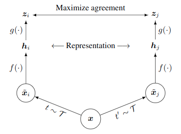
SimCLR实际上是Geoffrey Hinton和谷歌合作的论文A Simple Framework for Contrastive Learning of Visual Representations，严格来说他是一个自监督算法，不过我这里也把他归入半监督中了，他实际上是先无监督预训练然后进行监督微调的。

算法理论

SimCLR实际上是提出了一个简单的表征一致性学习框架。我觉得他的想法能work主要靠下面三点：

1. 有效的数据增强策略
2. 隐含层表征一致性损失约束
3. 超大batchsize

总体框架如下：

其中给定一个无标签样本\(x\)，从数据增强策略中采样两个数据增强操作\(t,t' \sim \mathcal{T}\)，分别应用到\(x\)得到\(\hat{x}_i,\hat{x}_j\)。论文中使用res50作为模型骨干\(f(\cdot)\)，得到中间表征\(\boldsymbol{h}_i,\boldsymbol{h}_j\)，接着论文指出在得到了中间表征不要直接用，再加个非线性投影头(nonlinear projection head)\(g(\cdot)\)更好,其实这个非线性投影头就是两个全连接层。下一步通过投影头得到了投影表征\(\boldsymbol{z}_i,\boldsymbol{z}_j\)，最后对投影表征计算对比损失(contrastive loss)，我更愿意称为一致性损失。

对比损失(contrastive loss)定义如下：

\[ \begin{aligned} \text{Let} \text{sim}(\boldsymbol{u},\boldsymbol{v})&=\frac{\boldsymbol{u}^T\boldsymbol{v}}{\parallel\boldsymbol{u}\parallel\parallel\boldsymbol{v}\parallel}\\ \mathcal{l}_{i,j}&=-\log \frac{\exp(\text{sim}(\frac{\boldsymbol{z}_i,\boldsymbol{z}_j}{\tau}))}{\sum_{k=1}^{2N}\mathcal{1}_{[k\neq i]}\exp(\text{sim}(\frac{\boldsymbol{z}_i,\boldsymbol{z}_k}{\tau}))} \end{aligned} \]

看起来和交叉熵不一样，但就是交叉熵。。。他的定义是是两个对应位置的图像投影表征內积应该越大越好，其他位置应该越小越好。下面代码部分我会讲的更详细些。

总算法流程图：

代码

因为他这个代码跑起来就得要imagenet，我懒得弄了，所以只看了最重要的损失部分的代码，不过还是按流程来讲。

数据输入

def map_fn(image, label):
  """Produces multiple transformations of the same batch."""
  if FLAGS.train_mode == 'pretrain':
    xs = []
    for _ in range(2):  # Two transformations
      # 预训练的时候是同一张图像
      xs.append(preprocess_fn_pretrain(image))
    image = tf.concat(xs, -1) # [h,w,2*c]
    label = tf.zeros([num_classes])
  else:
    image = preprocess_fn_finetune(image)
    label = tf.one_hot(label, num_classes)
  return image, label, 1.0

在无监督预训练的时候对于同一张图像执行两次数据增强，然后concat为[h,w,2*c]的图像。

# Split channels, and optionally apply extra batched augmentation.
# 前面变成了[h,w,2*c]，这里再拆分出来
features_list = tf.split(
    features, num_or_size_splits=num_transforms, axis=-1)
if FLAGS.use_blur and is_training and FLAGS.train_mode == 'pretrain':
  # 再做一些数据增强
  features_list = data_util.batch_random_blur(
      features_list, FLAGS.image_size, FLAGS.image_size)
# 现在变成了(num_transforms * bsz, h, w, c)
features = tf.concat(features_list, 0)  # (num_transforms * bsz, h, w, c)

注意他这里的features实际上还是图像，因为之前是[h,w,2*c]的形状，他这里重新分离的同时再分别加了一些数据增强，得到了[n*batch, h, w, c]的数据。

投影获取

with tf.variable_scope('base_model'):
  if FLAGS.train_mode == 'finetune' and FLAGS.fine_tune_after_block >= 4:
    # Finetune just supervised (linear) head will not update BN stats.
    model_train_mode = False
  else:
    # Pretrain or finetuen anything else will update BN stats.
    model_train_mode = is_training
  hiddens = model(features, is_training=model_train_mode)

# Add head and loss.
if FLAGS.train_mode == 'pretrain':
  tpu_context = params['context'] if 'context' in params else None
  hiddens_proj = model_util.projection_head(hiddens, is_training)

图像输入到basemodel得到隐含层输出，再通过投影头得到隐含层投影hiddens_proj。

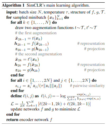
对比损失计算

def add_contrastive_loss(hidden,
                         hidden_norm=True,
                         temperature=1.0,
                         tpu_context=None,
                         weights=1.0):
  """Compute loss for model.

  Args:
    hidden: hidden vector (`Tensor`) of shape (bsz, dim).
    hidden_norm: whether or not to use normalization on the hidden vector.
    temperature: a `floating` number for temperature scaling.
    tpu_context: context information for tpu.
    weights: a weighting number or vector.

  Returns:
    A loss scalar.
    The logits for contrastive prediction task.
    The labels for contrastive prediction task.
  """
  # Get (normalized) hidden1 and hidden2.
  if hidden_norm:
    hidden = tf.math.l2_normalize(hidden, -1)
  hidden1, hidden2 = tf.split(hidden, 2, 0)
  batch_size = tf.shape(hidden1)[0]

  # Gather hidden1/hidden2 across replicas and create local labels.
  if tpu_context is not None:
    hidden1_large = tpu_cross_replica_concat(hidden1, tpu_context)
    hidden2_large = tpu_cross_replica_concat(hidden2, tpu_context)
    enlarged_batch_size = tf.shape(hidden1_large)[0]
    # TODO(iamtingchen): more elegant way to convert u32 to s32 for replica_id.
    replica_id = tf.cast(tf.cast(xla.replica_id(), tf.uint32), tf.int32)
    labels_idx = tf.range(batch_size) + replica_id * batch_size
    labels = tf.one_hot(labels_idx, enlarged_batch_size * 2)
    masks = tf.one_hot(labels_idx, enlarged_batch_size)
  else:
    hidden1_large = hidden1
    hidden2_large = hidden2
    labels = tf.one_hot(tf.range(batch_size), batch_size * 2)
    masks = tf.one_hot(tf.range(batch_size), batch_size)
  
  logits_aa = tf.matmul(hidden1, hidden1_large, transpose_b=True) / temperature
  logits_aa = logits_aa - masks * LARGE_NUM 
  logits_bb = tf.matmul(hidden2, hidden2_large, transpose_b=True) / temperature
  logits_bb = logits_bb - masks * LARGE_NUM 
  logits_ab = tf.matmul(hidden1, hidden2_large, transpose_b=True) / temperature
  logits_ba = tf.matmul(hidden2, hidden1_large, transpose_b=True) / temperature

  loss_a = tf.losses.softmax_cross_entropy(
      labels, tf.concat([logits_ab, logits_aa], 1), weights=weights)
  loss_b = tf.losses.softmax_cross_entropy(
      labels, tf.concat([logits_ba, logits_bb], 1), weights=weights)
  loss = loss_a + loss_b

  return loss, logits_ab, labels

因为现在的隐含层投影前一半和后一半是对同一张图像的输出，所以拆分为hidden1, hidden2 = tf.split(hidden, 2, 0)，接下来是得到hidden1_large，这里其实我不是很懂tpu上会和gpu有多大区别，不过对于gpu来说hidden1_large = hidden1。

有了投影，接下来制作标签，标签实际是batch单位矩阵并上一个零矩阵，mask是单位矩阵，矩阵的大小都是[batch,batch]，比如当batch=2时：

label = [[1., 0., 0., 0.],
        [0., 1., 0., 0.]] 

mask =  [[1., 0.],
        [0., 1.]] 

下面就是logits_aa,logits_bb，他们就是一个batch内的图像隐含层投影交叉做內积，而其中的对角线元素是相同向量做內积，那么因为他要做对比损失，希望将相似度转换成概率(越相似概率越大，越不相似概率越小)，向量自身的內积肯定是最大的(概率值最大)，所以这里就没有必要把对角线上的结果算到损失里面，他就利用mask将对角线相似度都减去一个极大值，将概率强行降为最小。

对于logits_ab,logits_ba，和上面一样类似，只不过现在的对角线元素是一张源图像两个不同增强后的表征投影向量內积(相似度)。

损失值就很明确了，即最大化一张源图像两个不同增强后的表征投影向量的相似度，最小化不同图像间表征投影向量的相似度，一张源图像一个增强的表征投影相似度被mask矩阵排除了。

思考

总的来说他的方法比我想的要简单好多，之前半监督学习里面对数据增强已经玩出花了，这里的数据增强只是简单的线性，都没有上数据增强策略。然后对于一致性学习这块，因为他神似交叉熵，而且他也考虑到了只用向量的夹角表示相似度(上面代码中有个hidden_norm选项)，这样实际上可以考虑和之前那些am softmax的论文结合起来，构建一个更严格的约束。