Explore AMX instructions: Unlock the performance of Apple Silicon
Since 2020, Apple has published M1/M2/M3. They have at least four different ways to perform high-intensity computing tasks.
Standard arm NEON instructions.
Undocumented AMX (Apple Matrix Co-processor) instructions. Issued by the CPU and performed on the co-processor.
Apple Neural Engine
Metal GPU
If we use ARM NEON instructions to accelerate the sgemm kernel on the single core of the M1 Max, It can achieve a performance of around 102 GFLOPS. But if use AMX instructions it can achieve 1475 GFLOPS!
In this article, I will introduce how you can leverage the AMX instructions to unlock the potential performance of Apple Silicon. And the all code I used in here (Verified on M2 Pro). This article refers to the work of Peter Cawley et al, which contains more instructions and usage methods.
1. Overview
A good one-image summary of AMX is the following figure from abandoned patent US20180074824A1. Consider a 32x32 grid of compute units, where each unit can perform 16-bit multiply-accumulate, or a 2x2 subgrid of units can perform 32-bit multiply-accumulate, or a 4x4 subgrid can perform 64-bit multiply-accumulate. To feed this grid, there is a pool of X registers each containing 32 16-bit elements (or 16 32-bit elements, or 8 64-bit elements) and a pool of Y registers similarly containing 32 16-bit elements (or 16 32-bit elements, or 8 64-bit elements). A single instruction can perform a full outer product: multiply every element of an X register with every element of a Y register, and accumulate with the Z element in the corresponding position.
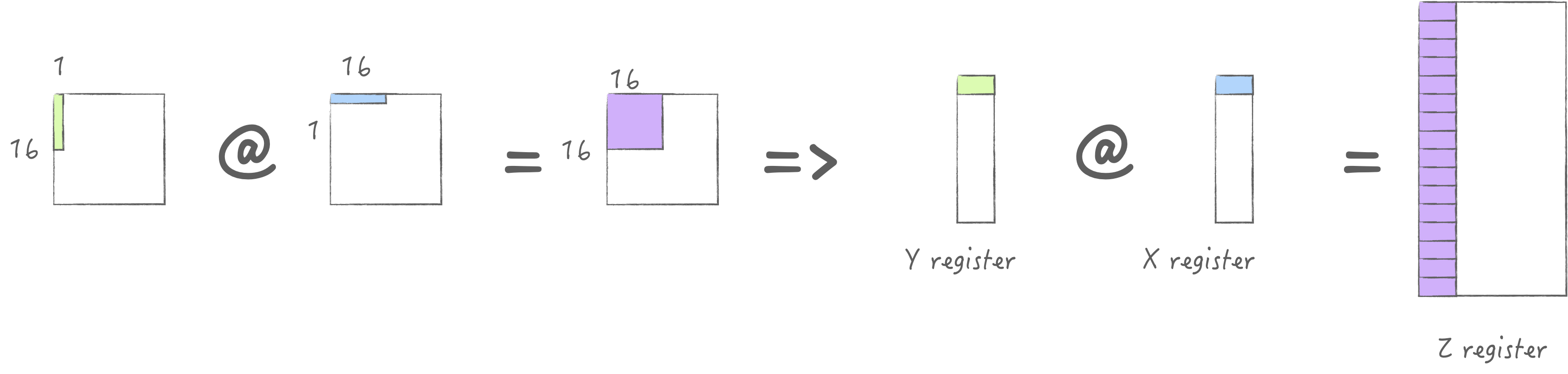
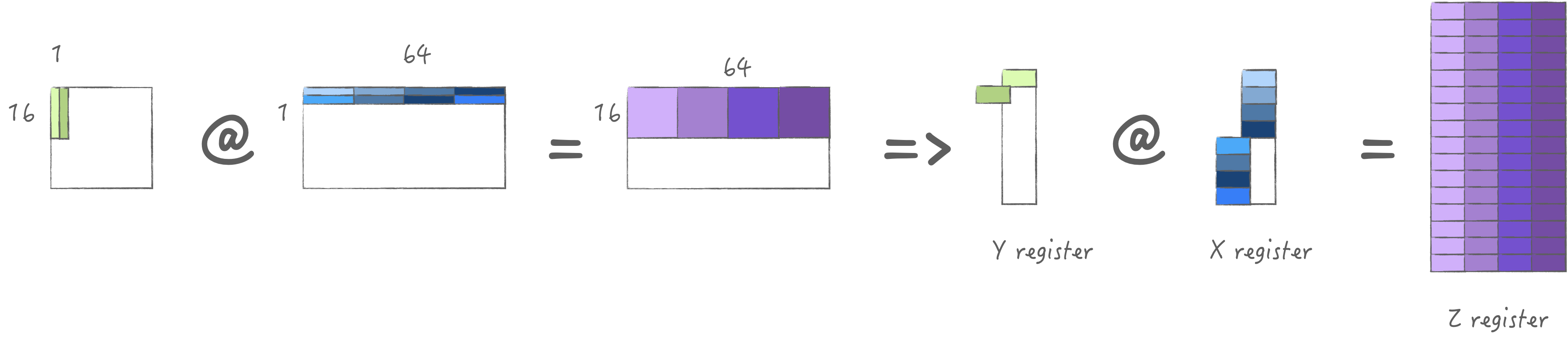
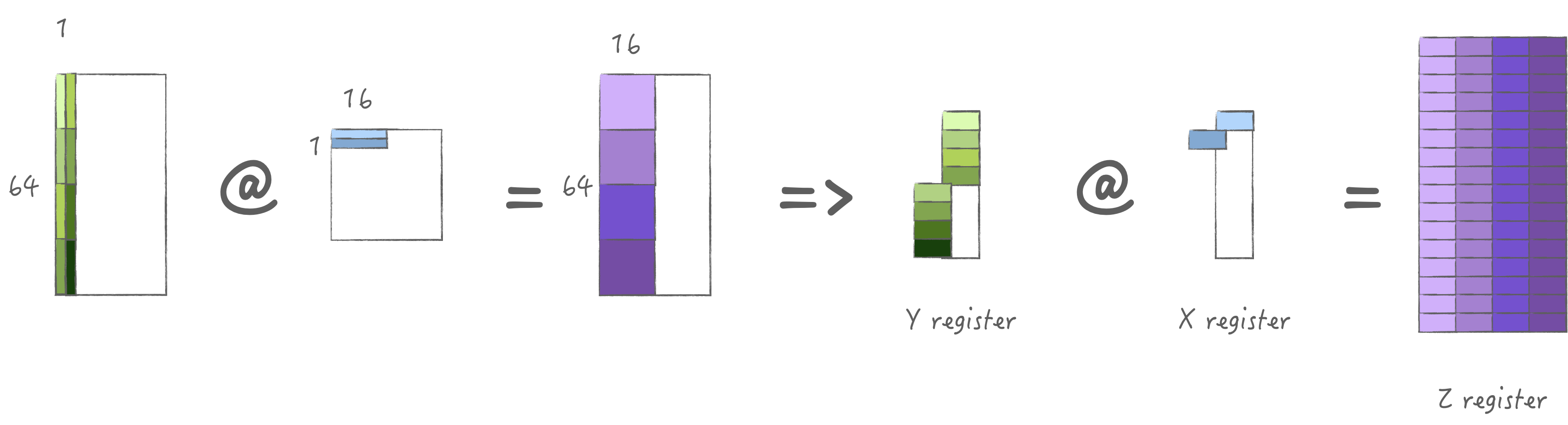
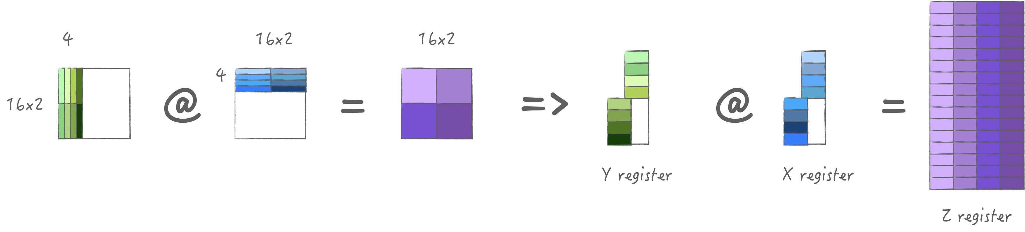
AMX provides LDX/LDY, FMA, LDZ/SDZ instructions. Where FMA has Matrix Mode and Vector Mode corresponding to outer product and inner product computation methods. The following two diagrams illustrate how the inner and outer products are calculated:
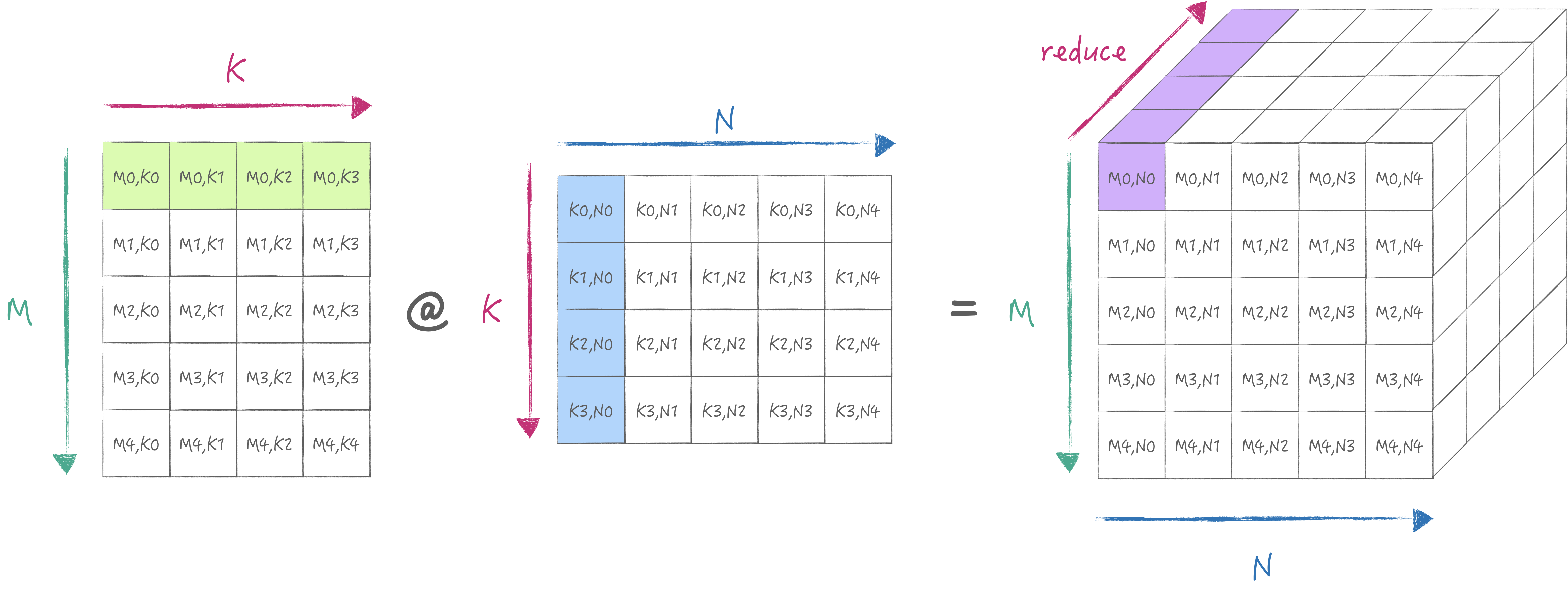
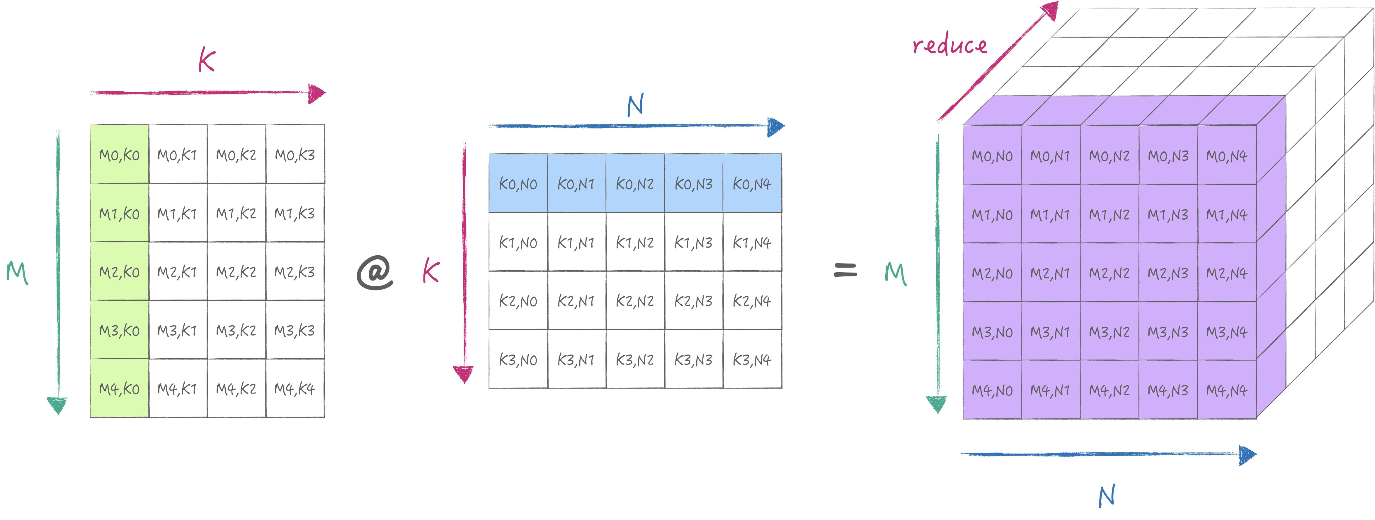
According to the diagrams, we know that the outer product has more hardware parallelism than the inner product.
2. Minimum Workflow
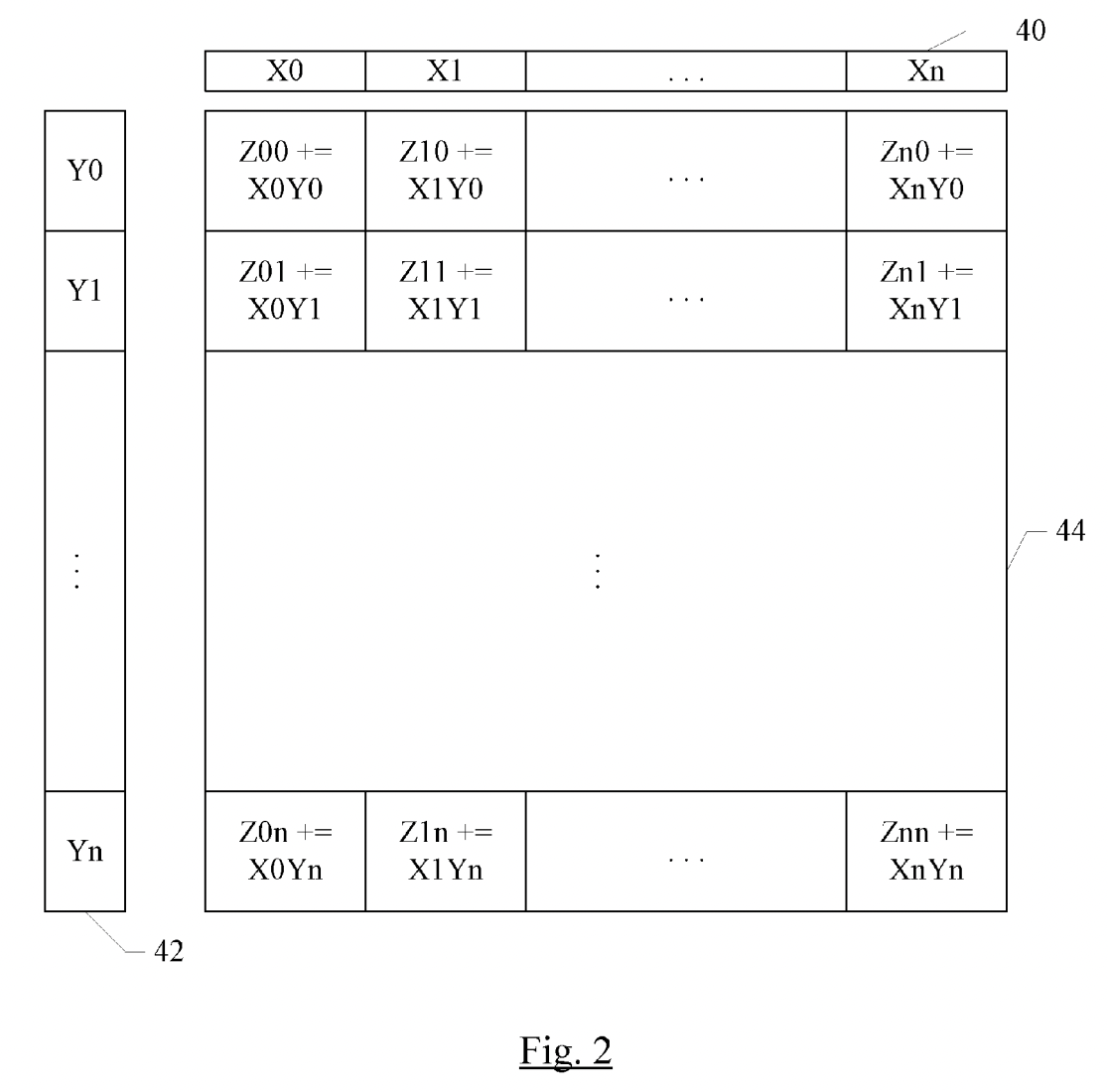
We also use one-image to explain the minimum calculation process and register specifications in AMX.
First, the X/Y register pool, each of them has 8 registers with a width of 64 bytes, can store data of type fp16/32/64 or i8/16/32, u8/16/32. Then there is the Z register pool, which has 64 registers with a width of 64 bytes, used to store the result of the outer product or inner product of the X/Y registers.
According to the description in the first section, the 2x2 cell subgrid performs 32-bit product, so 16 registers are required to perform the outer product, so the 64 registers are divided into 16 groups, and the interval of each group is 4 (64/16), that is, the outer product results are not stored continuously by register. (⚠️ AMX only supports loading and storage from main memory, and cannot be loaded and stored through general purpose registers/vector registers)
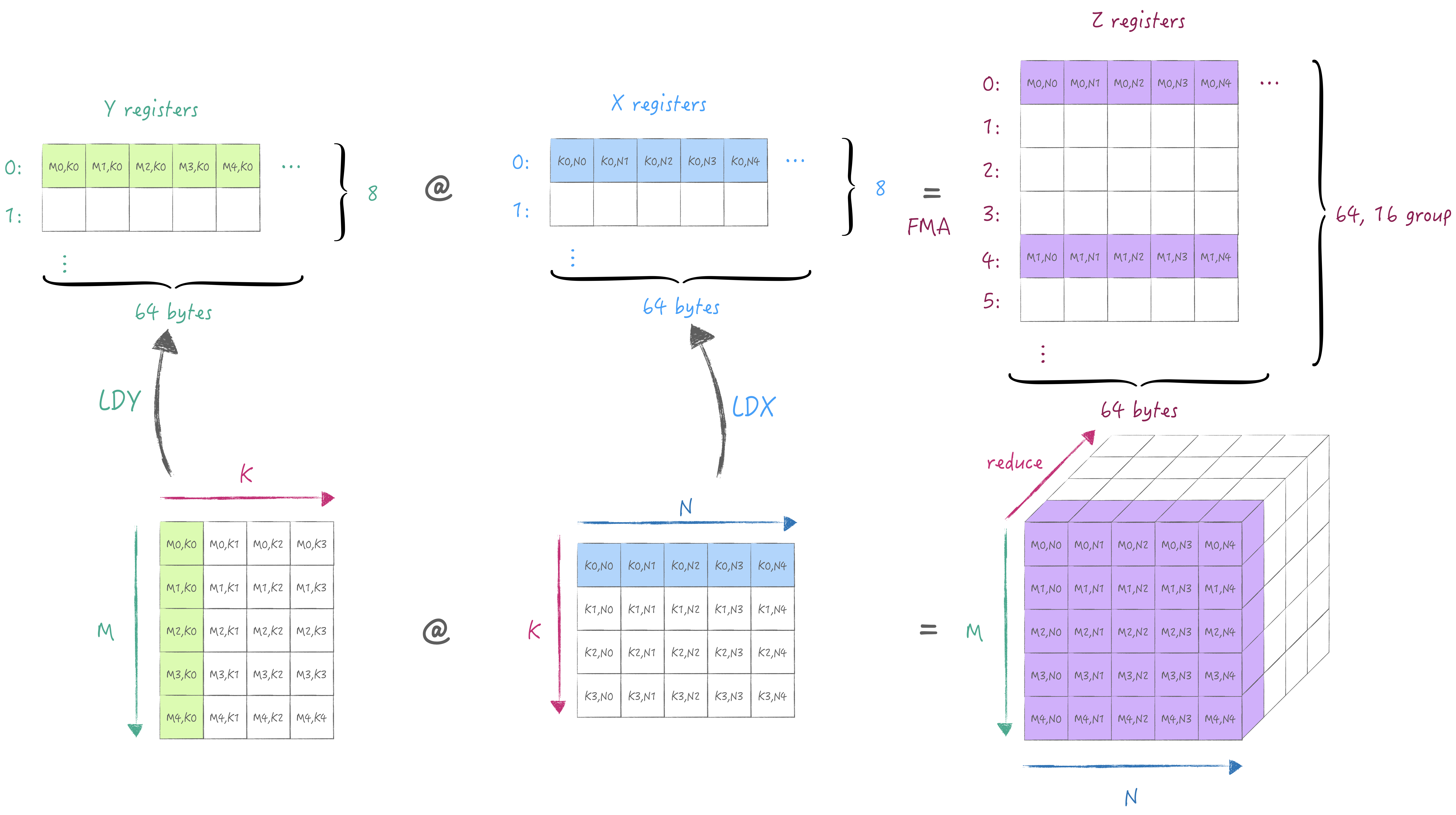
We can obtain a partial sum stored in the Z register pool through the outer product execution, and then we can switch the K dimension(matmul's reduction dimension) to accumulate the partial sum to get the complete result.
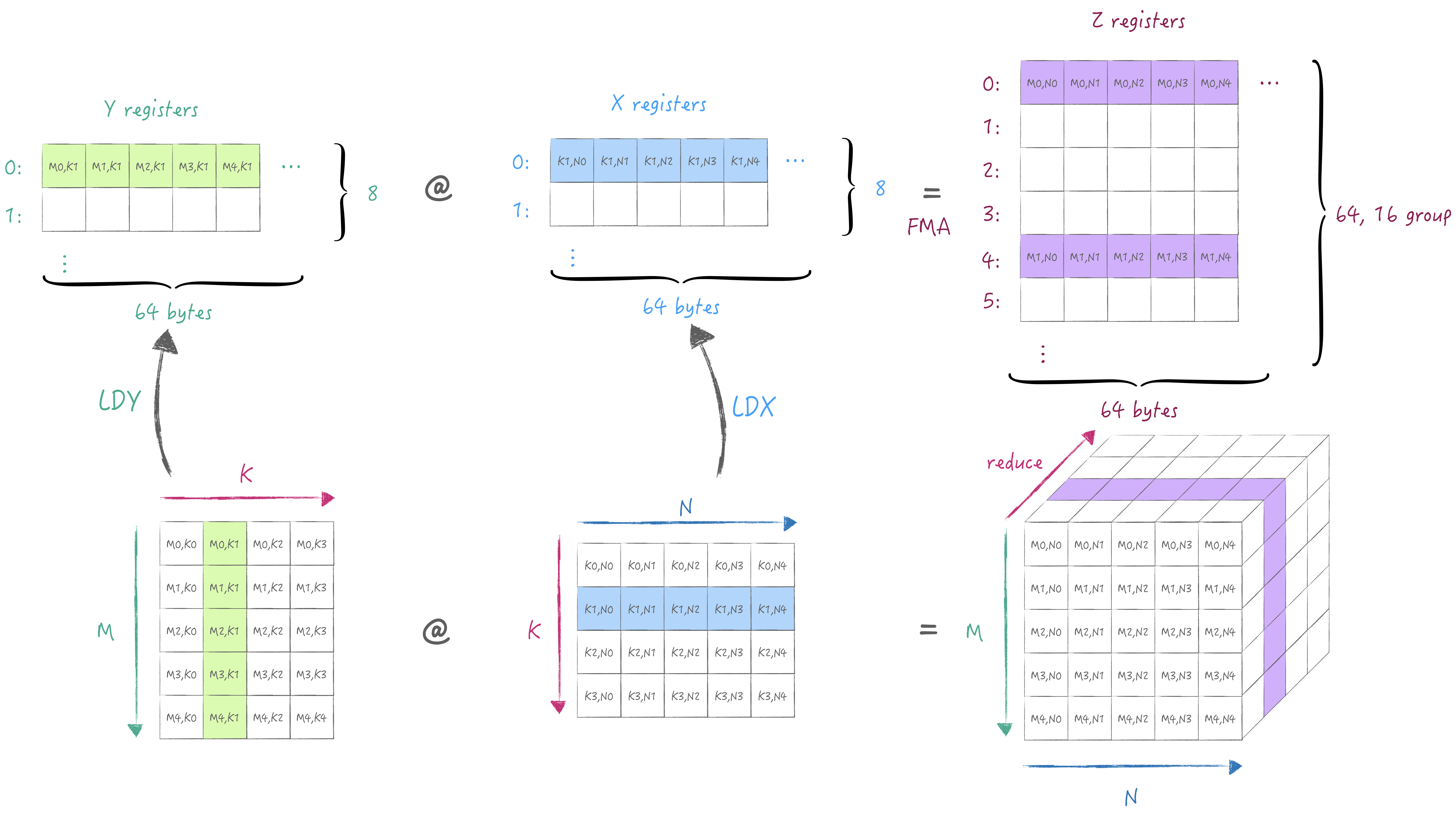
Reload the tile from A/B matrices of different K dimensions and then accumulate results to the same Z register group.
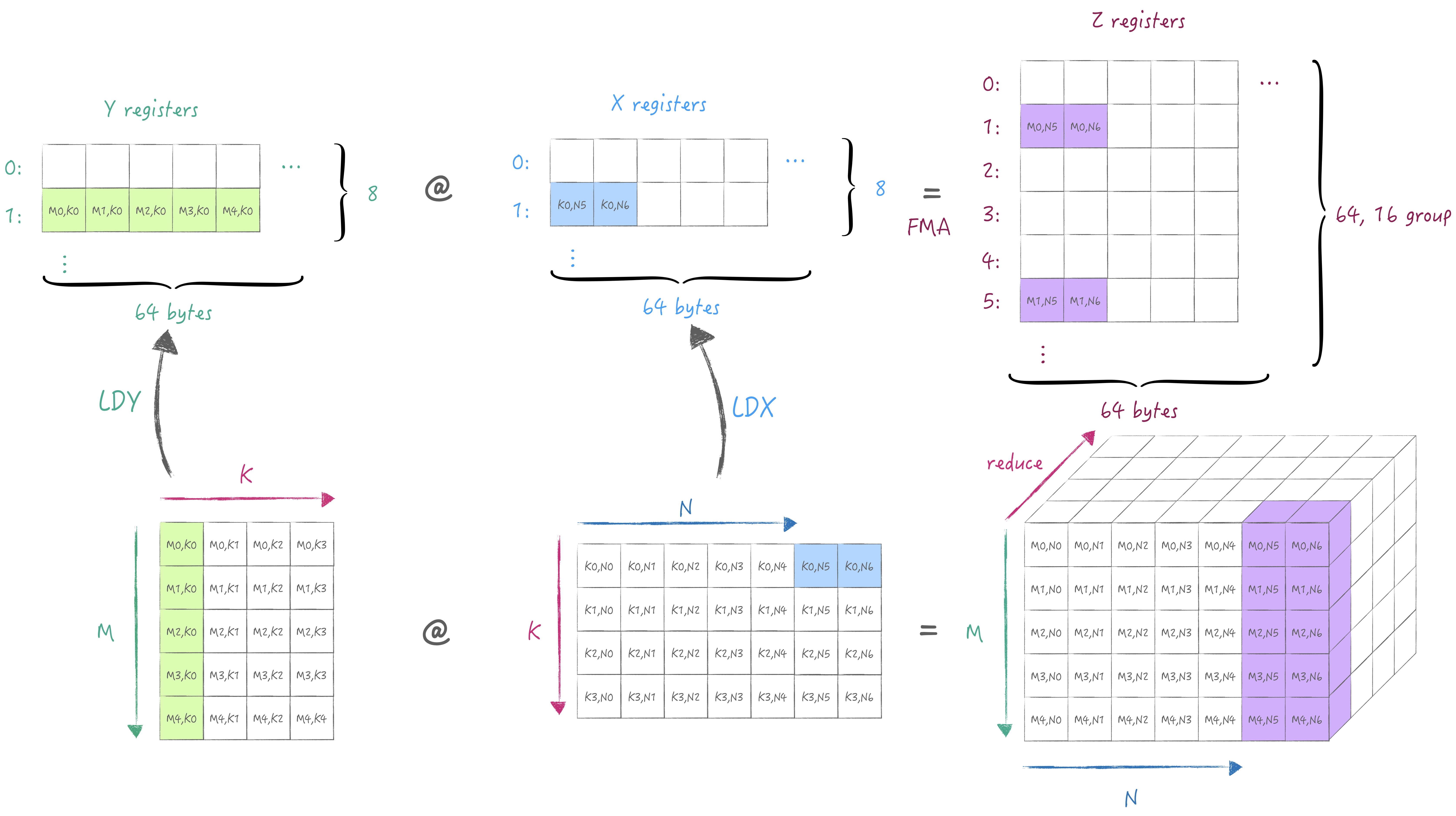
Or iterate the M/N dimension. In this example, we keep M unchanged and iterate to the next N. Meanwhile, we need to choose another group in the Z register pool to store the partial sum of the current M/N.
3. Theoretical Performance Metrics
In order to make good use of AMX, we must first understand the relevant metrics of AMX. So I have designed several tests to verify the theoretical performance metrics.
3.1 Computation Performance
From the previous section, we clearly know that the Z register group is divided into 16 groups in float32 datatype, and a computation results in a column in each group, so the ALU is actually divided into 4 groups. Here is to verify the peak performance of different ALU number enabled:
perf_func = [&z_nums]() { |
The results as following:
| ALU Nums | Gflop/s |
|---|---|
| 1 | 405.530 |
| 2 | 826.912 |
| 3 | 1244.570 |
| 4 | 1666.952 |
This shows that although each group of ALUs is individually configured and emitted, but they can be executed in parallel.
3.2 Load Performance
Here is the load performance test case I designed, where
reg nums represents the whether to load data into the X and
Y register at the same time. near indicates whether to read
consecutive addresses in memory. In M2 Pro, the l1 Dcache size is
65536, so K is designed larger than the l1
Dcache size. When near == 0, it needs to cross double cache
size to load data. width indicates the number of registers
used to read at once, The maximum number is 4 in M2.
constexpr size_t K = (65536 / 4 / (16 * 4)) * 4; |
After running this test, we have collected load performance metrics table:
| Reg Nums | Near | X Width | Y Width | GB/s |
|---|---|---|---|---|
| 1 | 1 | 1 | 0 | 87.1489 |
| 1 | 1 | 2 | 0 | 213.164 |
| 1 | 1 | 4 | 0 | 456.332 |
| 1 | 0 | 1 | 0 | 120.796 |
| 1 | 0 | 2 | 0 | 260.115 |
| 1 | 0 | 4 | 0 | 483.285 |
| 2 | 1 | 1 | 1 | 134.33 |
| 2 | 1 | 1 | 2 | 162.084 |
| 2 | 1 | 1 | 4 | 297.15 |
| 2 | 1 | 2 | 1 | 201.658 |
| 2 | 1 | 2 | 2 | 214.772 |
| 2 | 1 | 2 | 4 | 350.554 |
| 2 | 1 | 4 | 1 | 384.614 |
| 2 | 1 | 4 | 2 | 349.528 |
| 2 | 1 | 4 | 4 | 476.722 |
| 2 | 0 | 1 | 1 | 130.604 |
| 2 | 0 | 1 | 2 | 163.91 |
| 2 | 0 | 1 | 4 | 254.922 |
| 2 | 0 | 2 | 1 | 195.612 |
| 2 | 0 | 2 | 2 | 213.61 |
| 2 | 0 | 2 | 4 | 298.603 |
| 2 | 0 | 4 | 1 | 310.308 |
| 2 | 0 | 4 | 2 | 302.767 |
| 2 | 0 | 4 | 4 | 325.193 |
We can get some analysis from the table above. 1. increasing the
width can double the bandwidth, so this is a free lunch. 2.
consecutive reads is fast than non-consecutive reads, indicating we
should optimize the data layout. 3. loading two registers and loading
two groups in same register pool at the same time also not result in
bandwidth reduction, indicating that the A/B matrix can be loaded at the
same time.
3.3 Store Performance
Same like above, in store performance test also has
reg_num,near,width options. But
notice that the STZ instruction will store 16 groups from
the Z register pool at the same time.
constexpr size_t K = (65536 / 4 / (16 * 4)) * 2; |
Result:
| Reg Nums | Near | Width | GB/s |
|---|---|---|---|
| 1 | 1 | 1 | 10.3769 |
| 1 | 1 | 2 | 8.93052 |
| 1 | 0 | 1 | 12.9423 |
| 1 | 0 | 2 | 12.3377 |
| 2 | 1 | 1 | 5.69731 |
| 2 | 1 | 2 | 12.3658 |
| 2 | 0 | 1 | 7.55092 |
| 2 | 0 | 2 | 13.0133 |
| 3 | 1 | 1 | 6.58085 |
| 3 | 0 | 1 | 11.4118 |
| 4 | 1 | 1 | 8.8847 |
| 4 | 0 | 1 | 9.85956 |
It can be found that using multiple registers does not increase bandwidth, indicating that it is basically a serial store, but twice the width can still effectively increase bandwidth. However, the overall speed is several times slower than computing and loading, indicating that we cannot load and store Z frequently.
4. Design Micro Kernel
Based on the previous section's observation, we can trying to build the sgemm kernel. For efficiency, we design it according to the bottom-up principle. First we need to design a micro kernel that makes full use of the hardware's computing performance, then call the micro kernel in blocks to ensure the overall performance.
Review the most basic calculation process, load a column of M, load a row of N, and calculate a piece of MxN. it is obvious that the X/Y/Z register pool is not fully filled, especially the Z register pool, which means that only \(\frac{1}{4}\) is used, so the first goal is to use it up.
From the previous section, we know the maximum theoretical computational performance and bandwidth, so according to the formula we can calculate how many nanoseconds are needed for computation and loading.: \[ \begin{aligned} Compute Time &= \frac{FLOPs}{GFLOPS}\ ~NanoSeconds\\ Load Time &= \frac{Bytes}{GBS}\ ~NanoSeconds \end{aligned} \]
Next we design different calculation strategies based on the performance data and formulas.
4.1 Strategy 1: Load 1M and 4N
In my M2 Pro, AMX can load up to 4 * 64 bytes at a time,
so it can load 1 group of M and 4 groups of N,
and use the full 4 ALU for to get M * 4N, and then switch
different K in the next loop. In total, it is loaded once and calculated
4 times, and can only be cached once more due to the size limit of the X
register pool.
Looking up the table, we can see that the loading bandwidth is 297.15 GB/s, and the compute time and load time are respectively: \[ \begin{aligned} FLOPs &= 2 * M * N * ALU = 2 * 16 * 16 * 4 = 2048 \\ Compute Time &= FLOPs / 1666 = 1.229~NanoSeconds \\ Bytes &= (1 * M + 4 * N) * 4 = 320 \\ Load Time &= Bytes / 297.15 = 1.076~NanoSeconds \end{aligned} \]
The difference between they times is only 0.15ns, which
is not enough to load the data required for the next loop, causing the
ALU to fail to working continuously.
4.2 Strategy 2: Load 4M and 1N
Similar to the previous strategy, but there is an additional problem
here that the column direction of the A matrix is non-contiguous, and it
needs to be transposed 4 times M by the CPU before loading,
so it is not considered.
4.3 Strategy 3: Load 2M and 2N
In order to balance the storage usage of X/Y registers, we consider
loading M/N of the same size, that is, loading 2 groups. We can
calculate 4 times to get the 2M * 2N
output.
In my M2 Pro, the maximum loaded data is 4 * 64 bytesat
a time, so if load 2M and 2N of two different K, it means that can
actually be calculated 8 times, maximizing the utilization
of ALU. And we can prepare the next loop's input data in a free space of
the X/Y register pools.
Look up the table and get a bandwidth of 476.722 GB/s, which is taken into the formula to calculate: \[ \begin{aligned} FLOPs &= 2 * M * N * 4 * 2 = 4096 \\ Compute Time &= FLOPs / 1666 = 2.458~NanoSeconds \\ Bytes &= (4 * M + 4 * N) * 4 \\ Load Time &= Bytes / 476.722 = 1.074~NanoSeconds \end{aligned} \]
The compute time minus the load time is 1.384 ns, which
is greater than the next load time of 1.074 ns, indicating
that we can perfectly stream the computation, thus exerting the maximum
computing performance.
4.4 Verify Strategy 3
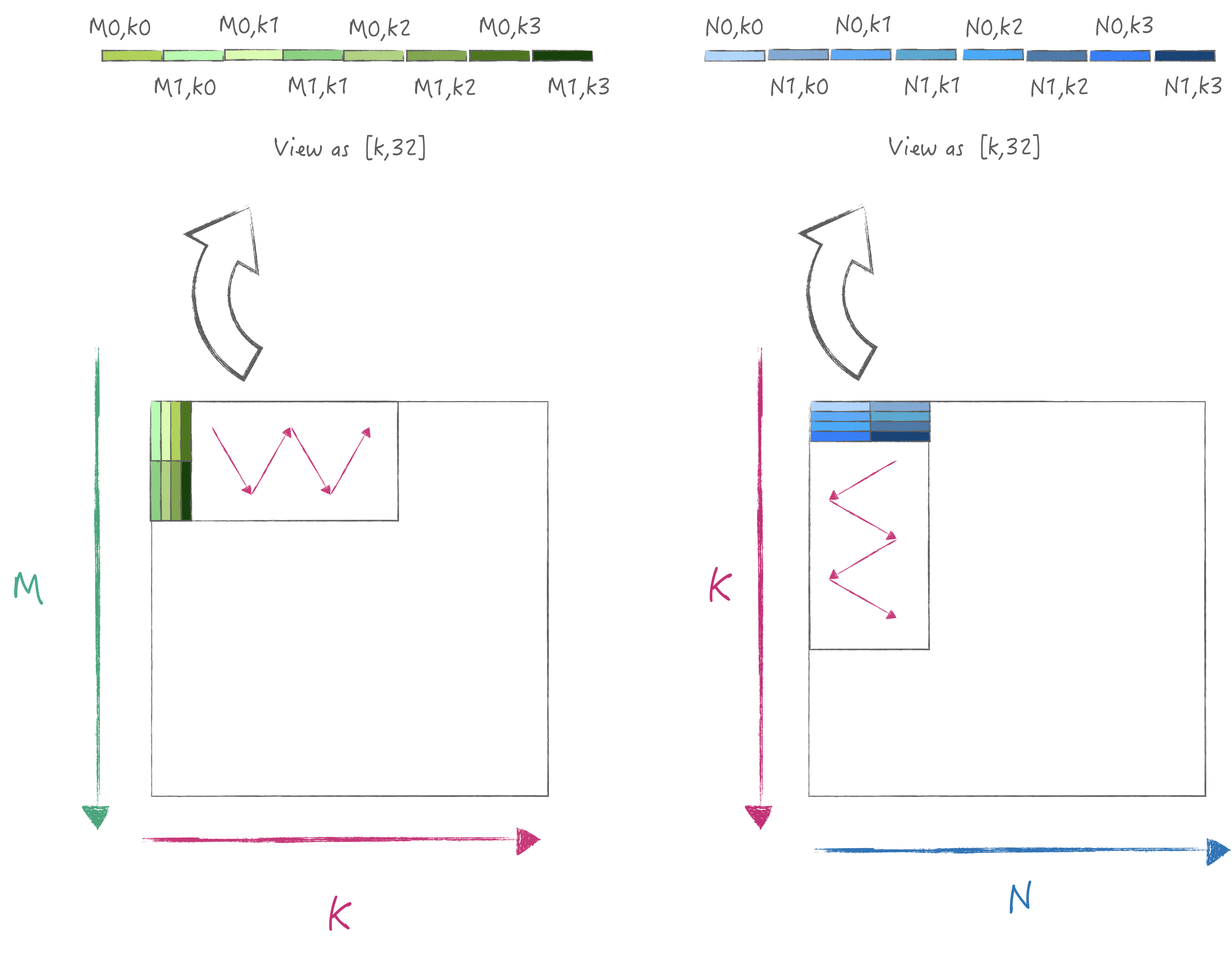
In order to achieve peak data loading performance, we need to
optimize the layout of the matrix, that is, pack the A/B matrix with a
width of 32, so that the loading is satisfied with contiguous memory
reading, and the result of 2 * M * N can be calculated at
one time. The specific iteration flowchart is as follows:
For the simplicity, I assume that M/K/N are multiples of the smallest
computing unit, and the input A/B matrix is required to be optimized for
layout. Here is the code: template <bool LoadC, bool StoreC, size_t KTile, size_t M, size_t N>
void gepdot(size_t curM, size_t curK, size_t curN,
const float packedA[KTile][32], const float packedB[KTile][32],
float C[M][N]) {
static_assert(KTile % 4 == 0, "not support k%4!=0");
if constexpr (LoadC) {
// load acc value.
for (size_t om = 0; om < 2; om++) {
for (size_t m = 0; m < 16; m++) {
AMX_STZ(
ldstz().row_index(m * 4 + om * 2).multiple().bind(C[om * 16 + m]));
}
}
}
for (size_t k = curK; k < curK + KTile; k += 4) {
for (size_t ok = k; ok < k + 4; ok += 2) {
// load [m0,k0], [m1,k0], [m0,k1], [m1,k1]
AMX_LDY(ldxy().register_index(0).multiple().multiple_four().bind(
(void *)packedA[ok]));
// load [n0,k0], [n1,k0], [n0,k1], [n1,k1]
AMX_LDX(ldxy().register_index(0).multiple().multiple_four().bind(
(void *)packedB[ok]));
// compute 8 times.
// [[m0,n0],[m0,n1],
// [m1,n0],[m1,n1]]
for (size_t ik = ok; ik < ok + 2; ik++) {
auto fma = ik == 0 ? fma32().skip_z() : fma32();
for (size_t m = 0; m < 2; m++) {
for (size_t n = 0; n < 2; n++) {
AMX_FMA32(fma.z_row(m * 2 + n)
.y_offset((ik - ok) * 2 * 16 * 4 + m * 16 * 4)
.x_offset((ik - ok) * 2 * 16 * 4 + n * 16 * 4));
}
}
}
}
}
// last time need store C.
if constexpr (StoreC) {
for (size_t om = 0; om < 2; om++) {
for (size_t m = 0; m < 16; m++) {
AMX_STZ(
ldstz().row_index(m * 4 + om * 2).multiple().bind(C[om * 16 + m]));
}
}
}
}
Tested under the conditions of
M = 16 * 2, K = 8192, N = 16 * 2, we obtained
1632.13 Gflop/s performance, reaching 97.9% of
the peak performance.
[----------] 1 test from test_amx |
5. Design Online Packing Scheme
If the layout of the input data is not optimized, then it is necessary to perform packing while considering the calculation. And in the example in the previous section, I did not set a large M and N, but in reality, I need to switch M and N, which brings another tiling size problem.
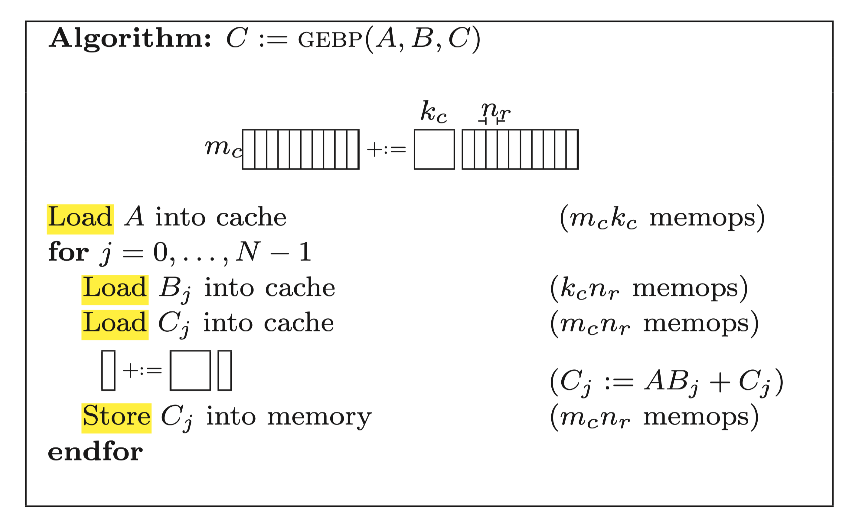
If we are using SIMD instructions for calculation, then a good online packing solution has been proposed in the paper Anatomy of High-Performance Matrix Multiplication:
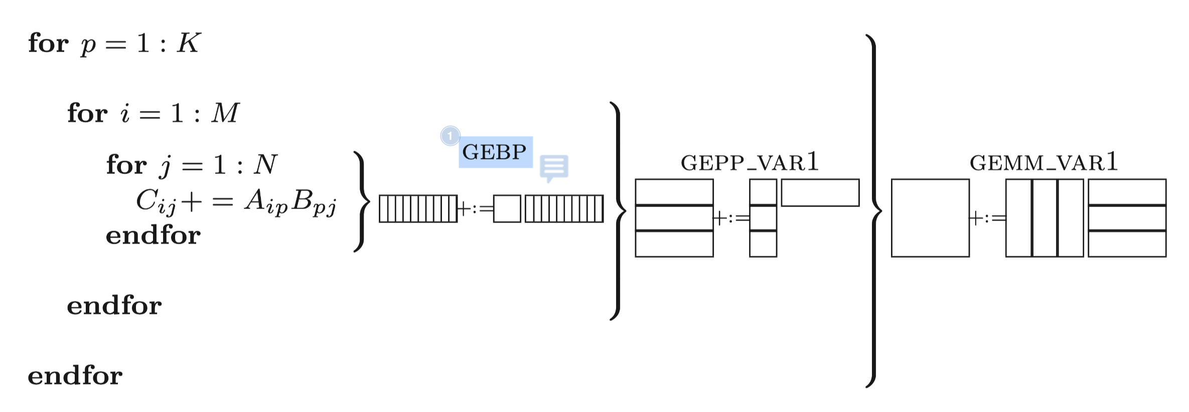
this paper choose the GEBP as micro kernel, However,
GEBP requires repeated load and store of the C matrix. For
CPU general purpose registers, its bandwidth is large enough. As long as
Nr is much larger than Kc, the memory overhead
of accessing the C matrix can be averaged.
But for AMX instructions, the bandwidth of the Z registers is only a few tenths of the bandwidth of the X/Y register, which obviously cannot be averaged. Therefore, we have to design a new method.
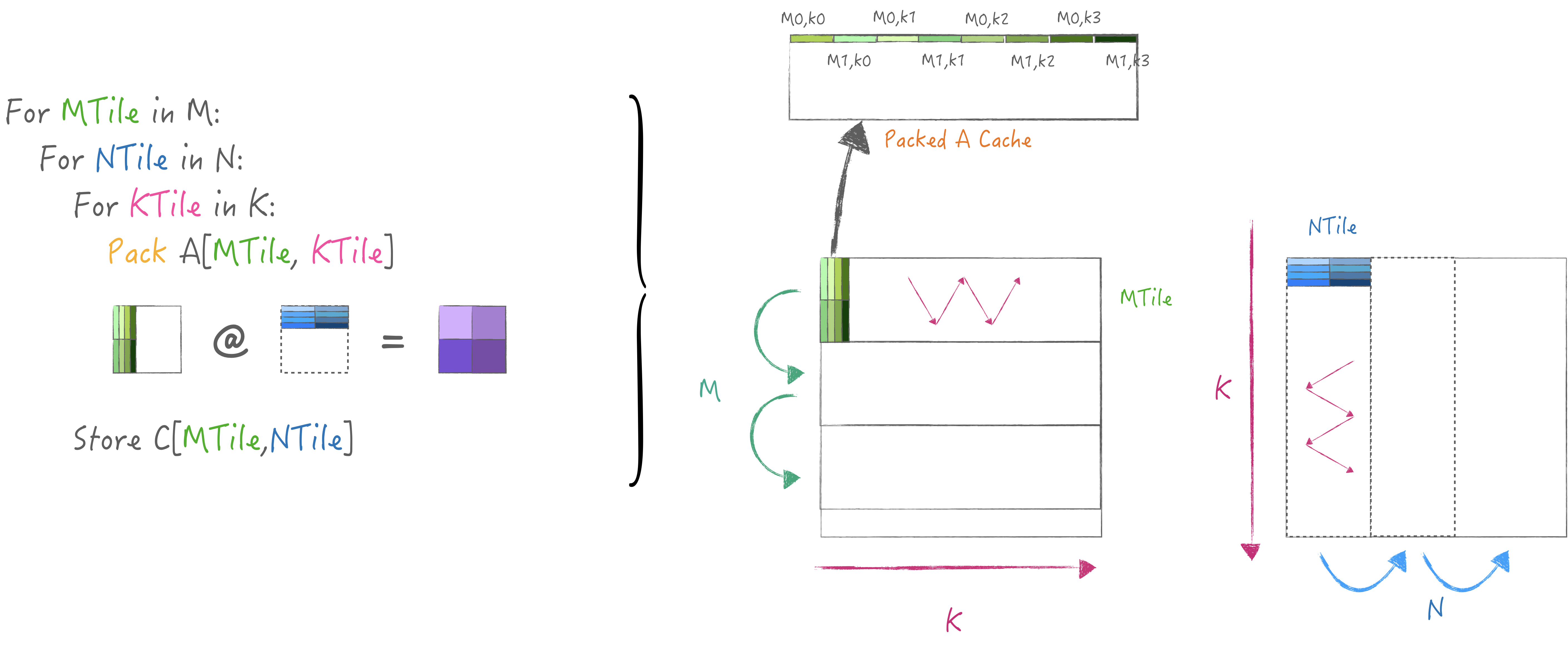
So I have implemented a simple two-level tiling strategy here. The
loop N in M is used to reuse the A matrix, and
the K dimension is placed in the innermost layer of the
loop to fit the gepdot kernel.
At the same time, a small piece of A is packed in each
KTile and cached, so that recompute can be avoided when
looping N:
final code: auto matmul = [&]() -> void {
constexpr size_t KTile = 32, MTile = 32, NTile = 32;
for (size_t mo = 0; mo < M; mo += MTile) {
float PackedA[K][MTile];
for (size_t no = 0; no < N; no += NTile) {
for (size_t ko = 0; ko < K; ko += KTile) {
// each time pack local innertile.
if (no == 0) {
for (size_t mi = 0; mi < MTile; mi++) {
for (size_t i = ko; i < ko + KTile; i++) {
PackedA[i][mi] = A[mo + mi][i];
}
}
}
gepdot_general<KTile, M, K, N>(false, (ko + KTile == K), mo, ko, no,
PackedA + ko, B, C);
}
}
}
};
The test performance achieved 70% of the performance of the libraries provided by Apple CBlas:
[ RUN ] test_amx.test_gepdot_general |
In fact, the strategy 3 is the bottleneck of the calculation, according to the theoretical performance value of the calculation of the pipeline after the actual remaining about "0.3ns" time can be assigned to the data load. Theoretically it can hidden the A matrix packing overhead, so as to reach the peak performance. So Beyond the Apple closed source library this challenging task to the readers 👻.
5. Further Questions
I have designed a test case to check whether AMX loading data updates
the cache: constexpr size_t K = (65536 / 4 / (16 * 2)) * 8; /* 65536 是cache size */
float N[1][16 * 2]{};
float M[K][16 * 2]{};
float *C = (float *)malloc(K * 65536);
auto func1 = [&N]() {
for (size_t i = 0; i < K; i++) {
AMX_LDX(ldxy().multiple().register_index(0).bind((void *)N[0]));
}
}
auto func2 = [&M]() {
for (size_t i = 0; i < K; i++) {
AMX_LDX(ldxy().multiple().register_index(0).bind((void *)M[i]));
}
}
auto func3 = [&C]() {
for (size_t i = 0; i < K; i++) {
AMX_LDX(
ldxy().multiple().register_index(0).bind((void *)(C + i * K)));
}
}
Where func1 always loads data at the same location,
func2 loads consecutive data in sequence, and
func3 loads data with a stride greater than l1 Dcache size
each time. The final result is as follows: func1: 29.9743 GB/s
func2: 219.201 GB/s
func3: 9.74711 GB/s
The results of func2 and func3 indicate
that the l1 Dcache is also important for AMX, but I can't understand the
difference between func1 and func2.
Theoretically, the accessed data should be cached in the cache, but from
the results, it seems that the cached data is the data behind the
current loading address. This question may require readers who know more
about the architecture to answer.