Probabilistic
Programming and Bayesian Methods for Hackers Chapter 3
Table of Contents
Opening the black box of MCMC
The Bayesian landscape
Exploring the landscape using the MCMC
Why Thousands of Samples?
Algorithms to perform MCMC
Other aproximation solutions to the posterior
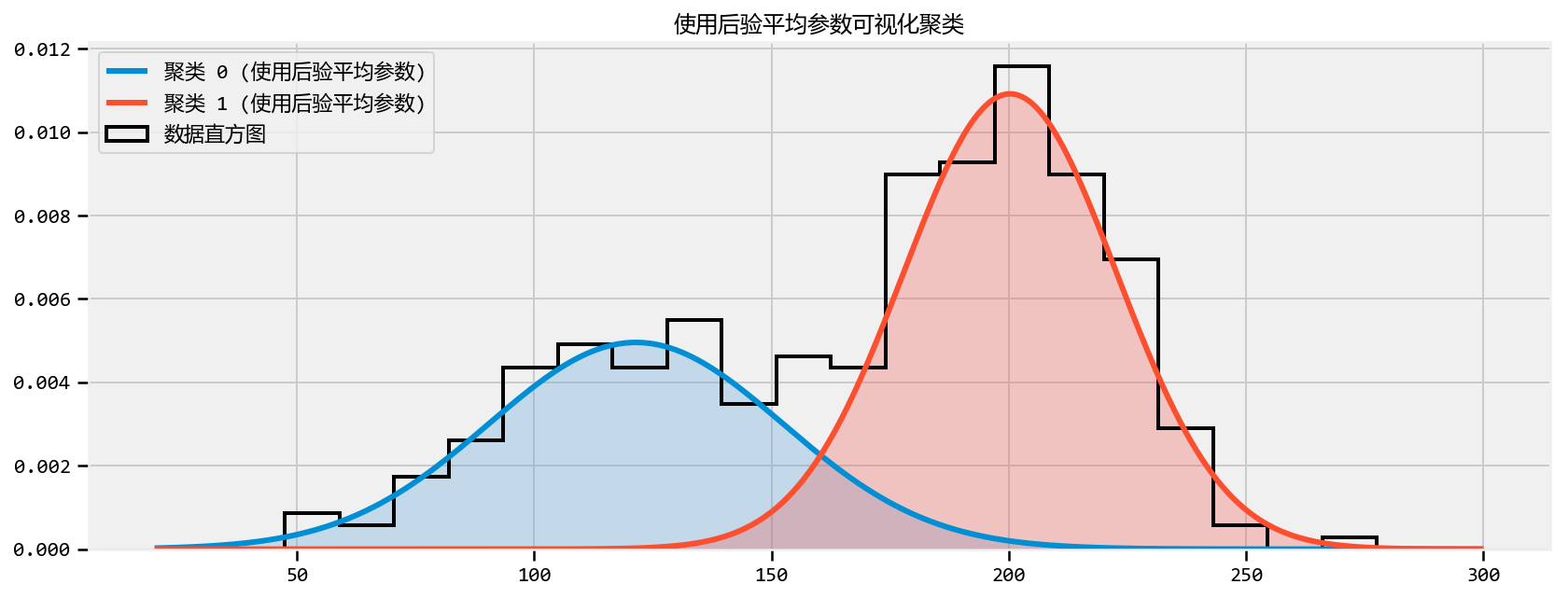
Example: Unsupervised Clustering Using a Mixture Model
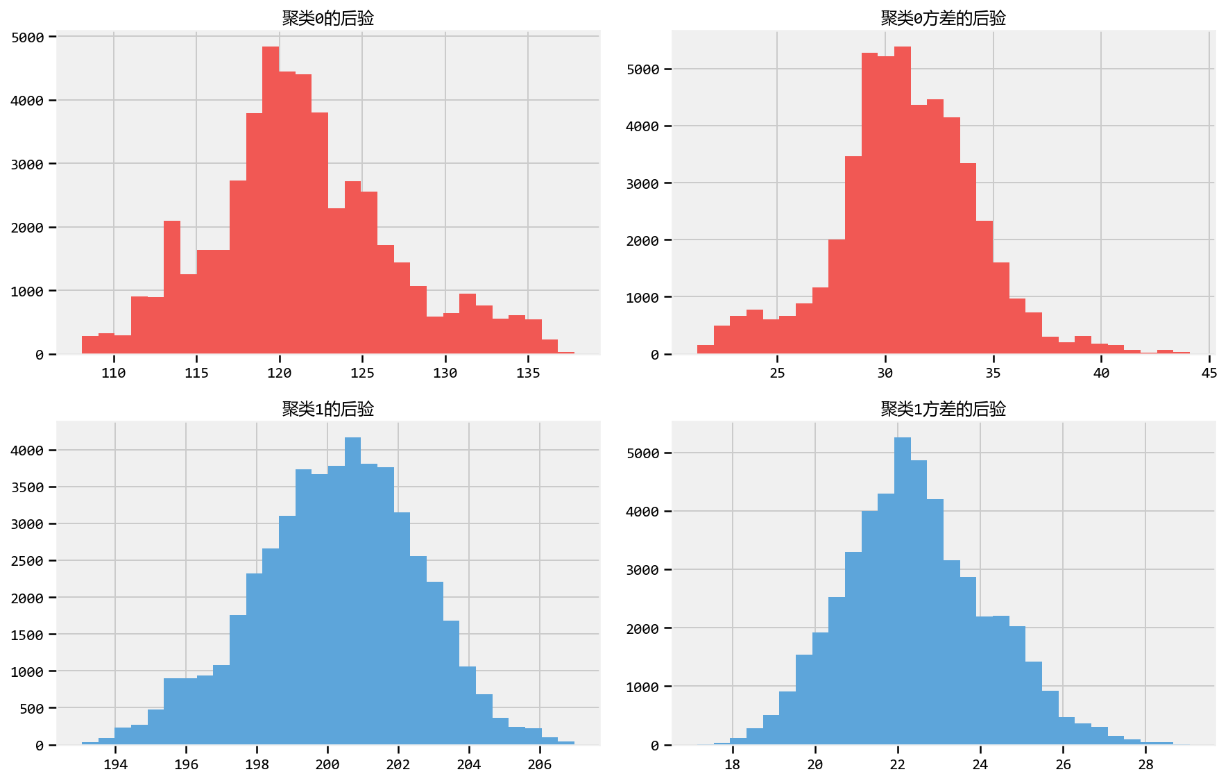
Cluster Investigation
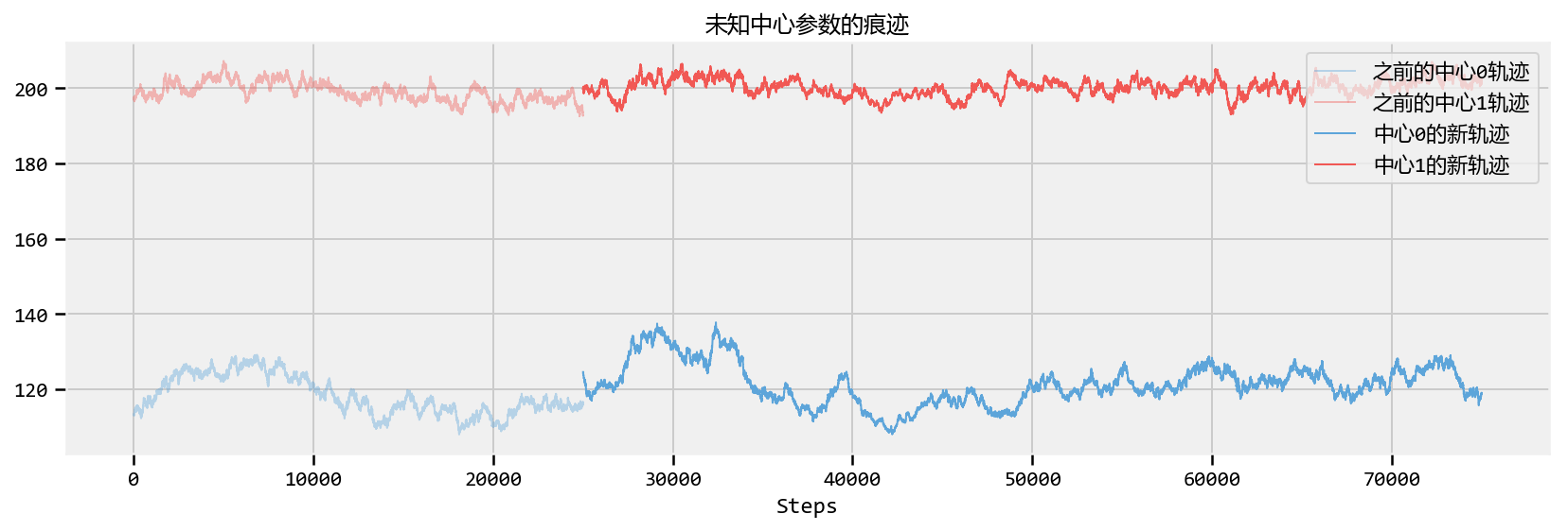
Important: Don't mix posterior samples
Returning to Clustering: Prediction
Diagnosing Convergence
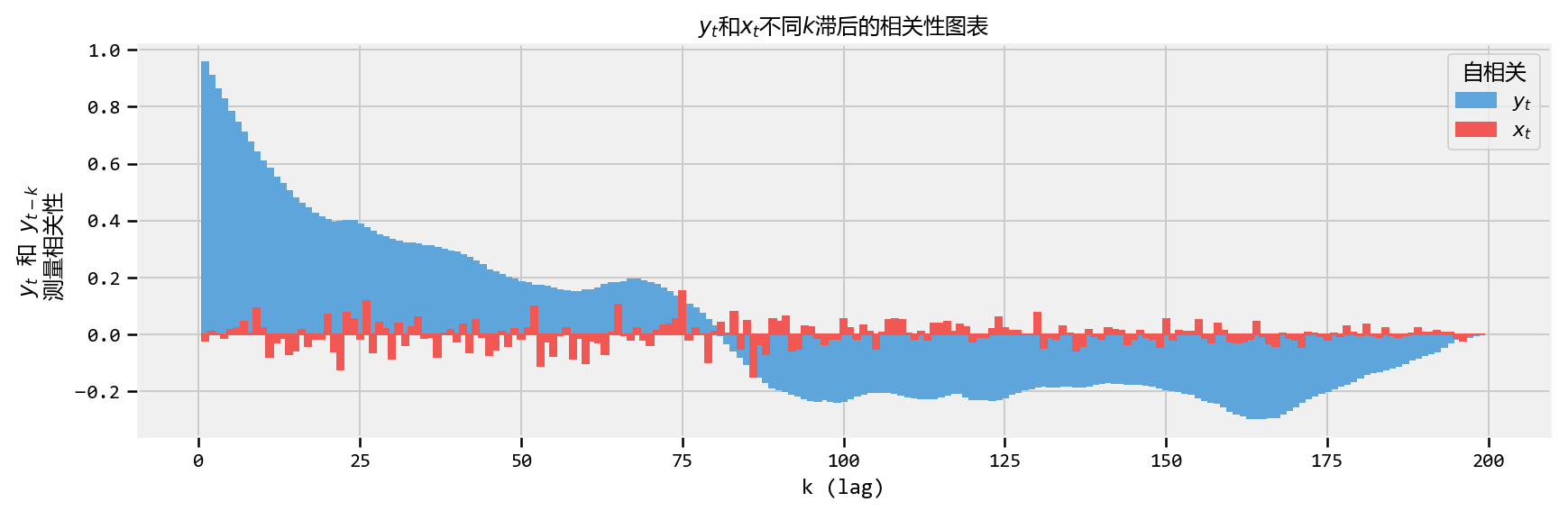
Autocorrelation
How does this relate to MCMC convergence?
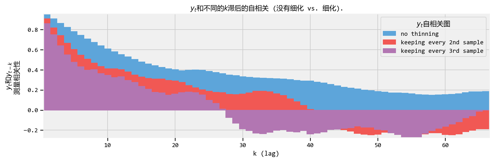
Thinning
Additional Plotting Options
Useful tips for MCMC
Intelligent starting values
Priors
Covariance matrices and eliminating parameters
The Folk Theorem of Statistical Computing
Conclusion
References
#@title Imports and Global Variables { display-mode: "form" } """ The book uses a custom matplotlibrc file, which provides the unique styles for matplotlib plots. If executing this book, and you wish to use the book's styling, provided are two options: 1. Overwrite your own matplotlibrc file with the rc-file provided in the book's styles/ dir. See http://matplotlib.org/users/customizing.html 2. Also in the styles is bmh_matplotlibrc.json file. This can be used to update the styles in only this notebook. Try running the following code: import json s = json.load(open("../styles/bmh_matplotlibrc.json")) matplotlib.rcParams.update(s) """ #@markdown This sets the warning status (default is `ignore`, since this notebook runs correctly) warning_status = "ignore"#@param ["ignore", "always", "module", "once", "default", "error"] import warnings warnings.filterwarnings(warning_status) with warnings.catch_warnings(): warnings.filterwarnings(warning_status, category=DeprecationWarning) warnings.filterwarnings(warning_status, category=UserWarning)
import numpy as np import os #@markdown This sets the styles of the plotting (default is styled like plots from [FiveThirtyeight.com](https://fivethirtyeight.com/)) matplotlib_style = 'fivethirtyeight'#@param ['fivethirtyeight', 'bmh', 'ggplot', 'seaborn', 'default', 'Solarize_Light2', 'classic', 'dark_background', 'seaborn-colorblind', 'seaborn-notebook'] import matplotlib as mpl import matplotlib.pyplot as plt; plt.style.use(matplotlib_style) import matplotlib.axes as axes; from matplotlib.patches import Ellipse from mpl_toolkits.mplot3d import Axes3D import pandas_datareader.data as web %matplotlib inline plt.rcParams['font.sans-serif']=['YaHei Consolas Hybrid'] import seaborn as sns; sns.set_context('notebook') from IPython.core.pylabtools import figsize #@markdown This sets the resolution of the plot outputs (`retina` is the highest resolution) notebook_screen_res = 'retina'#@param ['retina', 'png', 'jpeg', 'svg', 'pdf'] %config InlineBackend.figure_format = notebook_screen_res
import tensorflow as tf tfe = tf.contrib.eager
# Eager Execution #@markdown Check the box below if you want to use [Eager Execution](https://www.tensorflow.org/guide/eager) #@markdown Eager execution provides An intuitive interface, Easier debugging, and a control flow comparable to Numpy. You can read more about it on the [Google AI Blog](https://ai.googleblog.com/2017/10/eager-execution-imperative-define-by.html) use_tf_eager = False#@param {type:"boolean"}
# Use try/except so we can easily re-execute the whole notebook. if use_tf_eager: try: tf.enable_eager_execution() except: pass
import tensorflow_probability as tfp tfd = tfp.distributions tfb = tfp.bijectors
defevaluate(tensors): """Evaluates Tensor or EagerTensor to Numpy `ndarray`s. Args: tensors: Object of `Tensor` or EagerTensor`s; can be `list`, `tuple`, `namedtuple` or combinations thereof. Returns: ndarrays: Object with same structure as `tensors` except with `Tensor` or `EagerTensor`s replaced by Numpy `ndarray`s. """ if tf.executing_eagerly(): return tf.contrib.framework.nest.pack_sequence_as( tensors, [t.numpy() if tf.contrib.framework.is_tensor(t) else t for t in tf.contrib.framework.nest.flatten(tensors)]) return sess.run(tensors)
class_TFColor(object): """Enum of colors used in TF docs.""" red = '#F15854' blue = '#5DA5DA' orange = '#FAA43A' green = '#60BD68' pink = '#F17CB0' brown = '#B2912F' purple = '#B276B2' yellow = '#DECF3F' gray = '#4D4D4D' def__getitem__(self, i): return [ self.red, self.orange, self.green, self.blue, self.pink, self.brown, self.purple, self.yellow, self.gray, ][i % 9] TFColor = _TFColor()
defsession_options(enable_gpu_ram_resizing=True, enable_xla=True): """ Allowing the notebook to make use of GPUs if they're available. XLA (Accelerated Linear Algebra) is a domain-specific compiler for linear algebra that optimizes TensorFlow computations. """ config = tf.ConfigProto() config.log_device_placement = True if enable_gpu_ram_resizing: # `allow_growth=True` makes it possible to connect multiple colabs to your # GPU. Otherwise the colab malloc's all GPU ram. config.gpu_options.allow_growth = True if enable_xla: # Enable on XLA. https://www.tensorflow.org/performance/xla/. config.graph_options.optimizer_options.global_jit_level = ( tf.OptimizerOptions.ON_1) return config
defreset_sess(config=None): """ Convenience function to create the TF graph & session or reset them. """ if config isNone: config = session_options() global sess tf.reset_default_graph() try: sess.close() except: pass sess = tf.InteractiveSession(config=config)
reset_sess()
打开MCMC的黑匣子
前两章隐藏了TFP的内部机制,更常见的是来自读者的Markov Chain Monte
Carlo(MCMC)。包含本章的原因有三个方面。首先,任何关于贝叶斯推理的书都必须讨论MCMC。我不能打这个。责备统计学家。其次,了解MCMC的过程可以让您深入了解您的算法是否已融合(融合到什么?我们将达到这个目标)。第三,我们将理解为什么我们从后验返回了数千个样本作为解决方案,起初认为这可能是奇怪的。
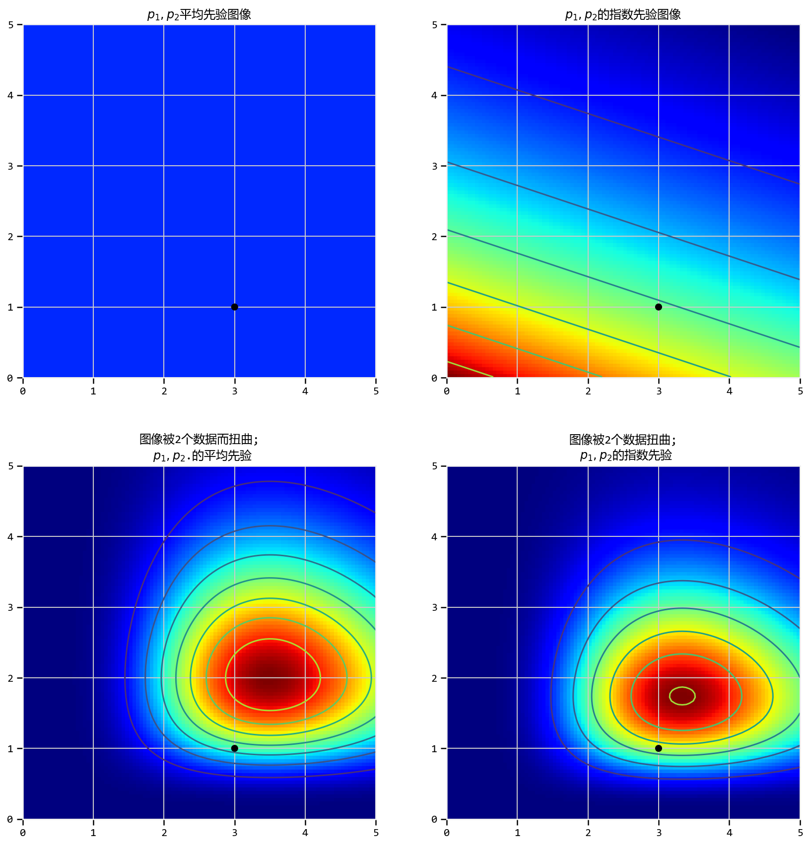
# SUBPLOT for Exponential + Data point plt.subplot(224) # This is the likelihood times prior, that results in the posterior. plt.contour(x_, y_, M_ * L_) im = plt.imshow(M_ * L_, interpolation='none', origin='lower', cmap=jet, extent=(0, 5, 0, 5))
我们应该探索我们先验表面和产生的变形后图像和观测数据,以找到后验。但是,我们不能天真地搜索空间:任何计算机科学家都会告诉你,在\(N\)中遍历\(N\)维空间是指数级的难度:当我们增加\(N\)时,空间的大小很快就会爆炸(the curse of
dimensionality)。我们有什么希望找到这些隐藏的山脉?
MCMC背后的想法是对空间进行智能搜索。说“搜索”意味着我们正在寻找一个特定的点,这可能不准确,因为我们真的在寻找一座宽阔的山峰。
# and to combine it with the observations: rv_observations = tfd.MixtureSameFamily( mixture_distribution=rv_assignments, components_distribution=tfd.Normal( loc=centers, scale=sds))
defjoint_log_prob(data_, sample_prob_1, sample_centers, sample_sds): """ Joint log probability optimization function. Args: data: tensor array representation of original data sample_prob_1: Scalar representing probability (out of 1.0) of assignment being 0 sample_sds: 2d vector containing standard deviations for both normal dists in model sample_centers: 2d vector containing centers for both normal dists in model Returns: Joint log probability optimization function. """ ### Create a mixture of two scalar Gaussians: rv_prob = tfd.Uniform(name='rv_prob', low=0., high=1.) sample_prob_2 = 1. - sample_prob_1 rv_assignments = tfd.Categorical(probs=tf.stack([sample_prob_1, sample_prob_2])) rv_sds = tfd.Uniform(name="rv_sds", low=[0., 0.], high=[100., 100.]) rv_centers = tfd.Normal(name="rv_centers", loc=[120., 190.], scale=[10., 10.]) rv_observations = tfd.MixtureSameFamily( mixture_distribution=rv_assignments, components_distribution=tfd.Normal( loc=sample_centers, # One for each component. scale=sample_sds)) # And same here. return ( rv_prob.log_prob(sample_prob_1) + rv_prob.log_prob(sample_prob_2) + tf.reduce_sum(rv_observations.log_prob(data_)) # Sum over samples. + tf.reduce_sum(rv_centers.log_prob(sample_centers)) # Sum over components. + tf.reduce_sum(rv_sds.log_prob(sample_sds)) # Sum over components. )
# Set the chain's start state. initial_chain_state = [ tf.constant(0.5, name='init_probs'), tf.constant([120., 190.], name='init_centers'), tf.constant([10., 10.], name='init_sds') ]
# Since MCMC operates over unconstrained space, we need to transform the # samples so they live in real-space. unconstraining_bijectors = [ tfp.bijectors.Identity(), # Maps R to R. tfp.bijectors.Identity(), # Maps R to R. tfp.bijectors.Identity(), # Maps R to R. ]
# Define a closure over our joint_log_prob. unnormalized_posterior_log_prob = lambda *args: joint_log_prob(data_, *args)
# Initialize the step_size. (It will be automatically adapted.) with tf.variable_scope(tf.get_variable_scope(), reuse=tf.AUTO_REUSE): step_size = tf.get_variable( name='step_size', initializer=tf.constant(0.5, dtype=tf.float32), trainable=False, use_resource=True )
# Sample from the chain. [ posterior_prob, posterior_centers, posterior_sds ], kernel_results = tfp.mcmc.sample_chain( num_results=number_of_steps, num_burnin_steps=burnin, current_state=initial_chain_state, kernel=hmc)
# Initialize any created variables. init_g = tf.global_variables_initializer() init_l = tf.local_variables_initializer()
W0727 20:52:11.363048 140336188528448 deprecation.py:323] From <ipython-input-31-144a4acba7c5>:39: make_simple_step_size_update_policy (from tensorflow_probability.python.mcmc.hmc) is deprecated and will be removed after 2019-05-22.
Instructions for updating:
Use tfp.mcmc.SimpleStepSizeAdaptation instead.
W0727 20:52:11.368744 140336188528448 deprecation.py:506] From <ipython-input-31-144a4acba7c5>:40: calling HamiltonianMonteCarlo.__init__ (from tensorflow_probability.python.mcmc.hmc) with step_size_update_fn is deprecated and will be removed after 2019-05-22.
Instructions for updating:
The `step_size_update_fn` argument is deprecated. Use `tfp.mcmc.SimpleStepSizeAdaptation` instead.
# Set the chain's start state. initial_chain_state = [ tf.to_float(1.) * tf.ones([], name='init_x', dtype=tf.float32), ]
# Initialize the step_size. (It will be automatically adapted.) with tf.variable_scope(tf.get_variable_scope(), reuse=tf.AUTO_REUSE): step_size = tf.get_variable( name='step_size', initializer=tf.constant(0.5, dtype=tf.float32), trainable=False, use_resource=True ) step_size_update_fn=tfp.mcmc.make_simple_step_size_update_policy(num_adaptation_steps=int(burnin * 0.8))
# Defining the HMC # Since we're only using one distribution for our simplistic example, # the use of the bijectors and unnormalized log_prob function is # unneccesary # # While not a good example of what to do if you have dependent # priors, this IS a good example of how to set up just one variable # with a simple distribution hmc=tfp.mcmc.HamiltonianMonteCarlo( target_log_prob_fn=tfd.Normal(name="rv_x", loc=tf.to_float(4.), scale=tf.to_float(1./np.sqrt(10.))).log_prob, num_leapfrog_steps=2, step_size=step_size, step_size_update_fn=step_size_update_fn, state_gradients_are_stopped=True)
在我们的例子中,$ A \(代表\) L_x = 1
\(和\) X \(是我们的证据:我们观察到\) x = 175 \(。对于我们后验分布的特定样本参数集\)(_0,_0,_1,_1,p)\(,我们有兴趣询问“\)x$在群集1
中的概率是否更大比它在集群0中的概率?“,其中概率取决于所选择的参数。
defautocorr(x): # from http://tinyurl.com/afz57c4 result = np.correlate(x, x, mode='full') result = result / np.max(result) return result[result.size // 2:]
在后验分布附近启动MCMC算法会很棒,因此开始正确采样将花费很少的时间。通过在“随机”变量创建中指定testval参数,我们可以通过告诉我们认为后验分布将在何处来帮助算法。在许多情况下,我们可以对参数进行合理的猜测。例如,如果我们有来自Normal分布的数据,并且我们希望估计$
$参数,那么一个好的起始值将是数据的* mean *。
mu = tfd.Uniform(name="mu", low=0., high=100.).sample(seed=data.mean())