Probabilistic
Programming and Bayesian Methods for Hackers Chapter 4
### Table of Contents - Dependencies & Prerequisites - The
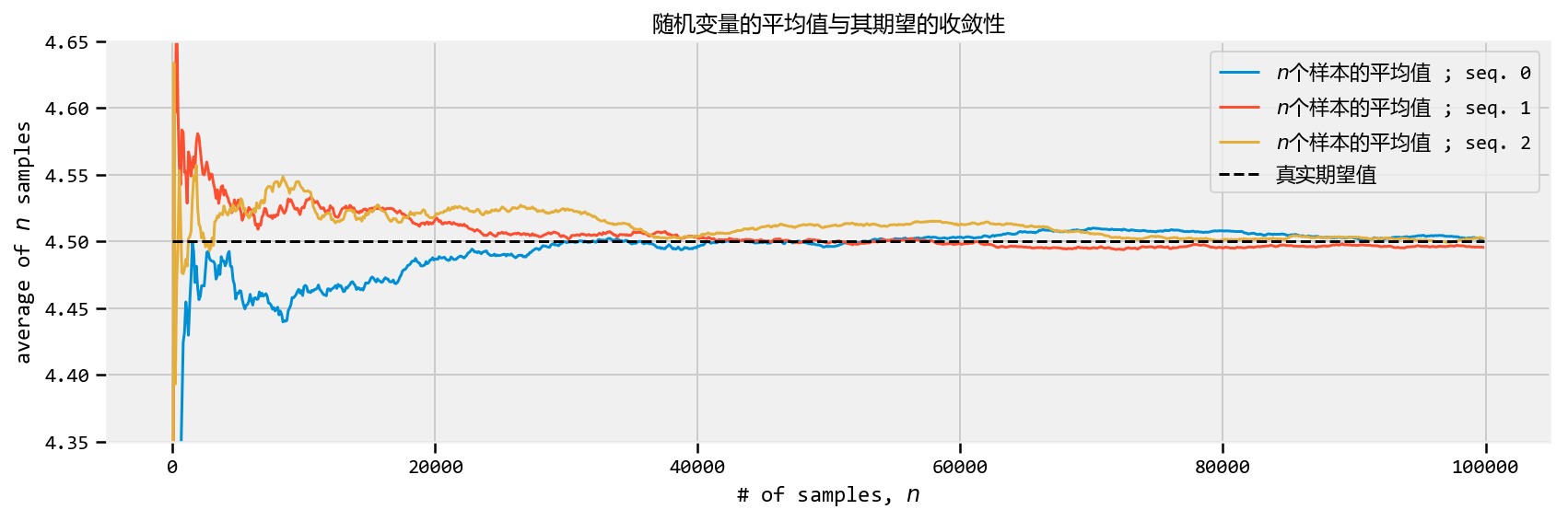
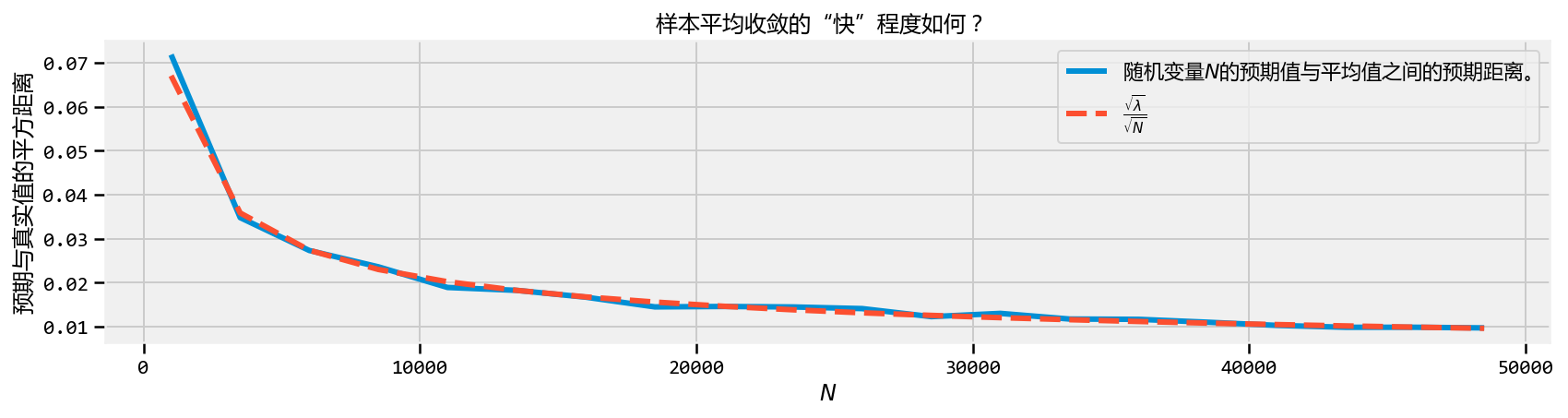
greatest theorem never told - The Law of Large Numbers - Intuition - How
do we compute \(Var(Z)\) though? -
Expected values and probabilities - What does this all have to do with
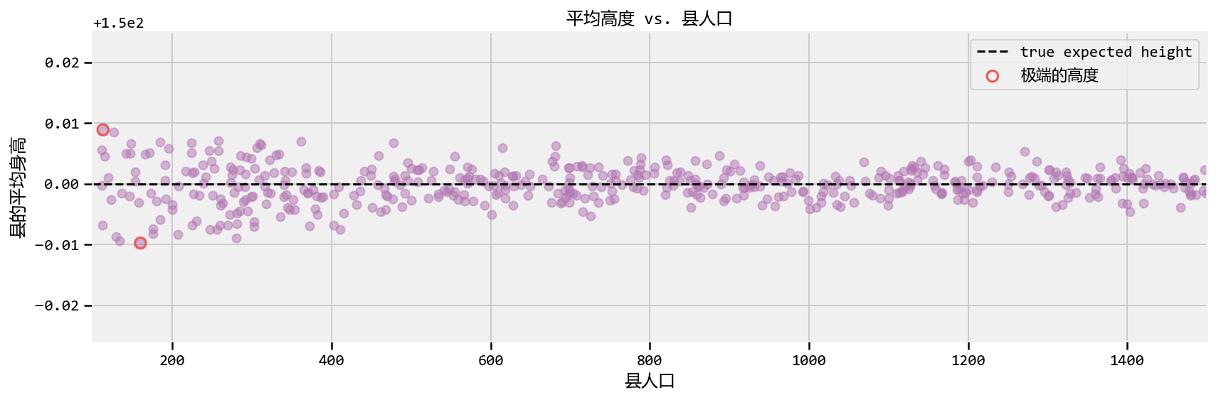
Bayesian statistics? - The Disorder of Small Numbers - Example:
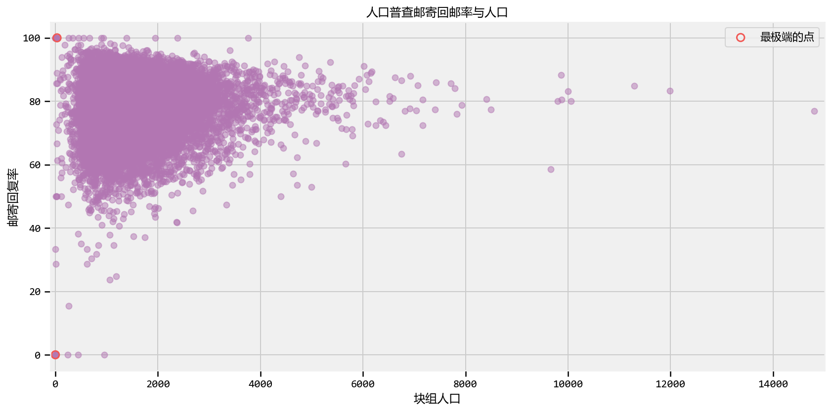
Aggregated geographic data - Example: Kaggle's U.S. Census Return Rate
Challenge - Example: How to order Reddit submissions - Setting up the
Praw Reddit API - Register your Application on Reddit - Reddit API Setup
- Sorting! - But this is too slow for real-time! - Extension to Starred
rating systems - Example: Counting Github stars - Conclusion - Appendix
- Exercises - Kicker Careers Ranked by Make Percentage - Average
Household Income by Programming Language - References
______
#@title Imports and Global Variables { display-mode: "form" } """ The book uses a custom matplotlibrc file, which provides the unique styles for matplotlib plots. If executing this book, and you wish to use the book's styling, provided are two options: 1. Overwrite your own matplotlibrc file with the rc-file provided in the book's styles/ dir. See http://matplotlib.org/users/customizing.html 2. Also in the styles is bmh_matplotlibrc.json file. This can be used to update the styles in only this notebook. Try running the following code: import json s = json.load(open("../styles/bmh_matplotlibrc.json")) matplotlib.rcParams.update(s) """ from __future__ import absolute_import, division, print_function
#@markdown This sets the warning status (default is `ignore`, since this notebook runs correctly) warning_status = "ignore"#@param ["ignore", "always", "module", "once", "default", "error"] import warnings warnings.filterwarnings(warning_status) with warnings.catch_warnings(): warnings.filterwarnings(warning_status, category=DeprecationWarning) warnings.filterwarnings(warning_status, category=UserWarning)
import numpy as np import os #@markdown This sets the styles of the plotting (default is styled like plots from [FiveThirtyeight.com](https://fivethirtyeight.com/)) matplotlib_style = 'fivethirtyeight'#@param ['fivethirtyeight', 'bmh', 'ggplot', 'seaborn', 'default', 'Solarize_Light2', 'classic', 'dark_background', 'seaborn-colorblind', 'seaborn-notebook'] import matplotlib.pyplot as plt; plt.style.use(matplotlib_style) import matplotlib.axes as axes; from matplotlib.patches import Ellipse from mpl_toolkits.mplot3d import Axes3D import pandas_datareader.data as web %matplotlib inline import seaborn as sns; sns.set_context('notebook') from IPython.core.pylabtools import figsize #@markdown This sets the resolution of the plot outputs (`retina` is the highest resolution) notebook_screen_res = 'retina'#@param ['retina', 'png', 'jpeg', 'svg', 'pdf'] %config InlineBackend.figure_format = notebook_screen_res plt.rcParams['font.sans-serif']=['YaHei Consolas Hybrid'] import tensorflow as tf tfe = tf.contrib.eager
# Eager Execution #@markdown Check the box below if you want to use [Eager Execution](https://www.tensorflow.org/guide/eager) #@markdown Eager execution provides An intuitive interface, Easier debugging, and a control flow comparable to Numpy. You can read more about it on the [Google AI Blog](https://ai.googleblog.com/2017/10/eager-execution-imperative-define-by.html) use_tf_eager = False#@param {type:"boolean"}
# Use try/except so we can easily re-execute the whole notebook. if use_tf_eager: try: tf.enable_eager_execution() except: pass
import tensorflow_probability as tfp tfd = tfp.distributions tfb = tfp.bijectors
defevaluate(tensors): """Evaluates Tensor or EagerTensor to Numpy `ndarray`s. Args: tensors: Object of `Tensor` or EagerTensor`s; can be `list`, `tuple`, `namedtuple` or combinations thereof. Returns: ndarrays: Object with same structure as `tensors` except with `Tensor` or `EagerTensor`s replaced by Numpy `ndarray`s. """ if tf.executing_eagerly(): return tf.contrib.framework.nest.pack_sequence_as( tensors, [t.numpy() if tf.contrib.framework.is_tensor(t) else t for t in tf.contrib.framework.nest.flatten(tensors)]) return sess.run(tensors)
class_TFColor(object): """Enum of colors used in TF docs.""" red = '#F15854' blue = '#5DA5DA' orange = '#FAA43A' green = '#60BD68' pink = '#F17CB0' brown = '#B2912F' purple = '#B276B2' yellow = '#DECF3F' gray = '#4D4D4D' def__getitem__(self, i): return [ self.red, self.orange, self.green, self.blue, self.pink, self.brown, self.purple, self.yellow, self.gray, ][i % 9] TFColor = _TFColor()
defsession_options(enable_gpu_ram_resizing=True, enable_xla=True): """ Allowing the notebook to make use of GPUs if they're available. XLA (Accelerated Linear Algebra) is a domain-specific compiler for linear algebra that optimizes TensorFlow computations. """ config = tf.ConfigProto() config.log_device_placement = True if enable_gpu_ram_resizing: # `allow_growth=True` makes it possible to connect multiple colabs to your # GPU. Otherwise the colab malloc's all GPU ram. config.gpu_options.allow_growth = True if enable_xla: # Enable on XLA. https://www.tensorflow.org/performance/xla/. config.graph_options.optimizer_options.global_jit_level = (tf.OptimizerOptions.ON_1) return config
defreset_sess(config=None): """ Convenience function to create the TF graph & session or reset them. """ if config isNone: config = session_options() global sess tf.reset_default_graph() try: sess.close() except: pass sess = tf.InteractiveSession(config=config)
reset_sess()
WARNING: Logging before flag parsing goes to stderr. W0728
19:21:27.291700 139811709552448 lazy_loader.py:50] The TensorFlow
contrib module will not be included in TensorFlow 2.0. For more
information, please see: *
https://github.com/tensorflow/community/blob/master/rfcs/20180907-contrib-sunset.md
* https://github.com/tensorflow/addons *
https://github.com/tensorflow/io (for I/O related ops) If you depend on
functionality not listed there, please file an issue.
defD_N(n): """ This function approx. D_n, the average variance of using n samples. """ Z = tfd.Poisson(rate=lambda_val_).sample(sample_shape=(int(n), int(N_Y_))) average_Z = tf.reduce_mean(Z, axis=0) average_Z_ = evaluate(average_Z) return np.sqrt(((average_Z_ - expected_value_)**2).mean())
for i,n inenumerate(N_array_): D_N_results_[i] = D_N(n)
# Our strategy to vectorize this problem will be to end-to-end concatenate the # number of draws we need. Then we'll loop over the pieces. d = tfp.distributions.Normal(loc=mean_height, scale= 1. / std_height) x = d.sample(np.sum(population_))
average_across_county = [] seen = 0 for p in population_: average_across_county.append(tf.reduce_mean(x[seen:seen+p])) seen += p average_across_county_full = tf.stack(average_across_county)
##located the counties with the apparently most extreme average heights. [ average_across_county_, i_min, i_max ] = evaluate([ average_across_county_full, tf.argmin( average_across_county_full ), tf.argmax( average_across_county_full ) ])
#plot population size vs. recorded average plt.scatter( population_, average_across_county_, alpha = 0.5, c=TFColor[6]) plt.scatter( [ population_[i_min], population_[i_max] ], [average_across_county_[i_min], average_across_county_[i_max] ], s = 60, marker = "o", facecolors = "none", edgecolors = TFColor[0], linewidths = 1.5, label="极端的高度")
# Github data scrapper # See documentation_url: https://developer.github.com/v3/
from json import loads import datetime import numpy as np from requests import get
""" variables of interest: indp. variables - language, given as a binary variable. Need 4 positions for 5 langagues - #number of days created ago, 1 position - has wiki? Boolean, 1 position - followers, 1 position - following, 1 position - constant dep. variables -stars/watchers -forks """
MAX = 8000000 today = datetime.datetime.today() randint = np.random.randint N = 10#sample size. auth = ("zhen8838", "zqh19960305" )
#define data matrix: X = np.zeros( (N , 12), dtype = int )
for i inrange(N): is_fork = True is_valid_language = False while is_fork == Trueor is_valid_language == False: is_fork = True is_valid_language = False params = {"since":randint(0, MAX ) } r = get("https://api.github.com/repositories", params = params, auth=auth ) results = loads( r.text )[0] #im only interested in the first one, and if it is not a fork. # print(results) is_fork = results["fork"] r = get( results["url"], auth = auth) #check the language repo_results = loads( r.text ) try: language_mappings[ repo_results["language" ] ] is_valid_language = True except: pass
1. How would you estimate the quantity \(E\left[ \cos{X} \right]\), where \(X \sim \text{Exp}(4)\)? What about \(E\left[ \cos{X} | X \lt 1\right]\), i.e.
the expected value given we know \(X\) is less than 1? Would you need more
samples than the original samples size to be equally accurate?
你如何估计$ E \(,其中\) X
(4)\(?或者\) E \(,即预期值*给定*我们知道\) X
$小于1?您是否需要比原始样本大小更多的样本才能同样准确?
## Enter code here import tensorflow as tf import tensorflow_probability as tfp tfd = tf.distributions
reset_sess()
exp = tfd.Exponential(rate=4.) N = 10000 X = exp.sample(sample_shape=int(N))
2. The following table was located in the paper "Going for Three:
Predicting the Likelihood of Field Goal Success with Logistic
Regression" [2]. The table ranks football field-goal kickers by their
percent of non-misses. What mistake have the researchers made?
Kicker Careers Ranked
by Make Percentage
Rank
Kicker
Make %
Number of Kicks
1
Garrett Hartley
87.7
57
2
Matt Stover
86.8
335
3
Robbie Gould
86.2
224
4
Rob Bironas
86.1
223
5
Shayne Graham
85.4
254
…
…
…
51
Dave Rayner
72.2
90
52
Nick Novak
71.9
64
53
Tim Seder
71.0
62
54
Jose Cortez
70.7
75
55
Wade Richey
66.1
56
In August 2013, a
popular post on the average income per programmer of different
languages was trending. Here's the summary chart: (reproduced without
permission, cause when you lie with stats, you gunna get the hammer).
What do you notice about the extremes?
Average
household income by programming language
Language
Average Household Income ($)
Data Points
Puppet
87,589.29
112
Haskell
89,973.82
191
PHP
94,031.19
978
CoffeeScript
94,890.80
435
VimL
94,967.11
532
Shell
96,930.54
979
Lua
96,930.69
101
Erlang
97,306.55
168
Clojure
97,500.00
269
Python
97,578.87
2314
JavaScript
97,598.75
3443
Emacs Lisp
97,774.65
355
C#
97,823.31
665
Ruby
98,238.74
3242
C++
99,147.93
845
CSS
99,881.40
527
Perl
100,295.45
990
C
100,766.51
2120
Go
101,158.01
231
Scala
101,460.91
243
ColdFusion
101,536.70
109
Objective-C
101,801.60
562
Groovy
102,650.86
116
Java
103,179.39
1402
XSLT
106,199.19
123
ActionScript
108,119.47
113
References
Wainer, Howard. The Most Dangerous Equation. American
Scientist, Volume 95.
Clarck, Torin K., Aaron W. Johnson, and Alexander J. Stimpson.
"Going for Three: Predicting the Likelihood of Field Goal Success with
Logistic Regression." (2013): n. page. Web.
20 Feb. 2013.